Summary:
Reduce min rate of WETH2 and WBTC markets to 0.1% and wstETH to 0.2% from 0.5%.
Abstract:
The IRM curve adjustments are a multi-part optimization that began with a reduction of min rate in the target markets from 2-3% to 0.5% in this proposal. Part 2 will further reduce min rate and will likely be followed by subsequent proposals to continue reducing the parameter over time.
Motivation:
We are proposing to reduce min rate in these markets because they are not configured for optimal market performance. In general, these markets equilibriate at a relatively low utilization that is more conservative than necessary and may impact the competitiveness of these markets. Our methodology identifies a safe target utilization based on historical supply drawdowns during volatile periods. Sim runs balance priority metrics including mean squared error, time above threshold, and rate/utilization volatility. Our simulations help identify IRM parameters that maximize market competitiveness without sacrificing sufficient liquidity availability.
We are implementing these adjustments in phases to minimize impact to market rates with a gradual approach. Since part 1 of these markets adjustments (executed on March 2), utilizations have increased from a range around 50% to low to mid-60%. The directionality justifies further optimization toward what we consider desirable market operation.
Analysis:
Our analyses are given below, showing in general a wider min/max spread in the target markets to achieve desired performance enhancements. These are shared for academic interest and provide insight into the trajectory of our recommended adjustment for these markets.
WETH-long2 Analysis
WETH-long2
The WETH-long2 market was deployed on ethereum with the controller address:0x23F5a668A9590130940eF55964ead9787976f2CC.
The current Interest Rate Model (IRM) is SemiLogIRM, with the following parameters:
-
min_rate= 0.005 -
max_rate= 0.7
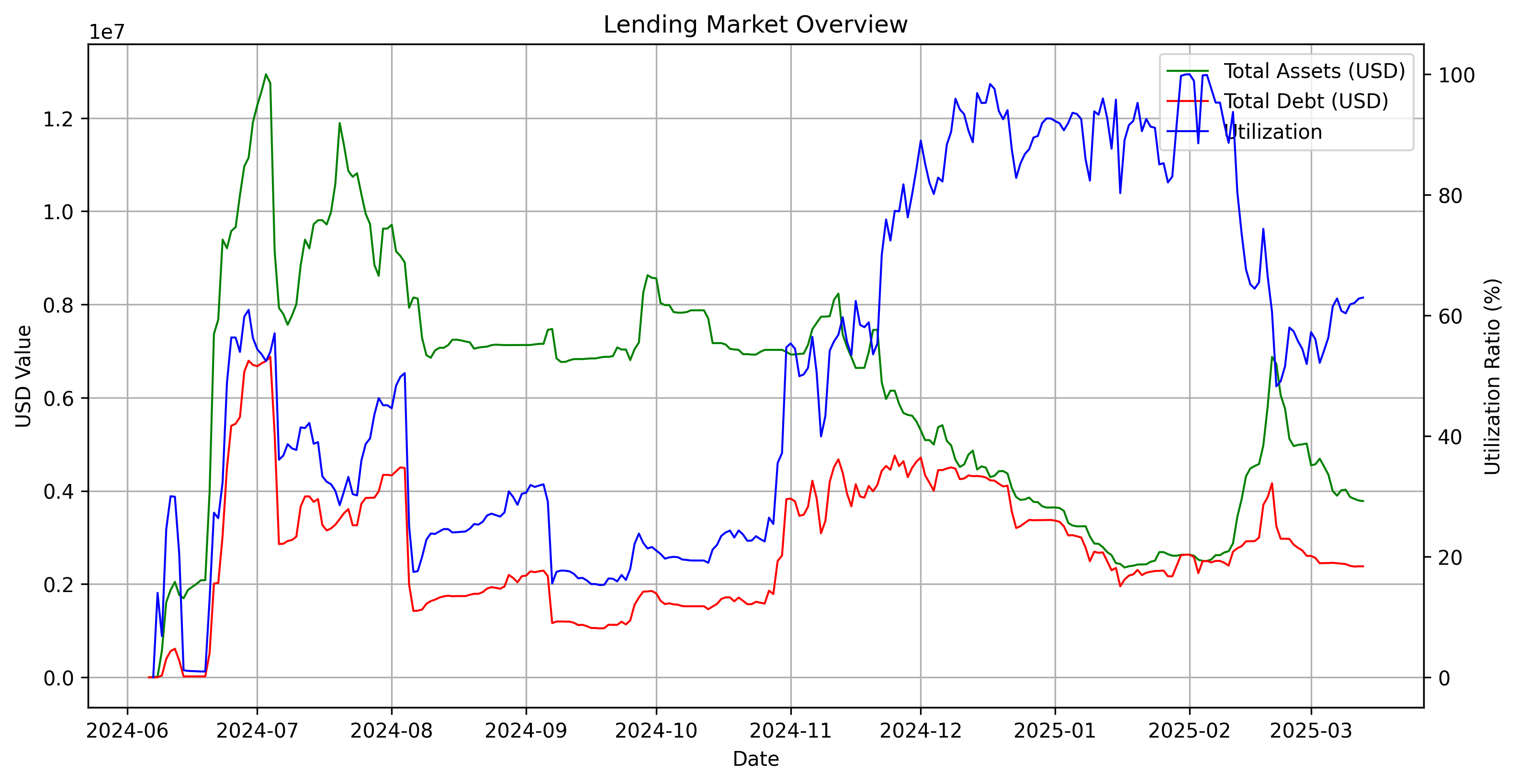
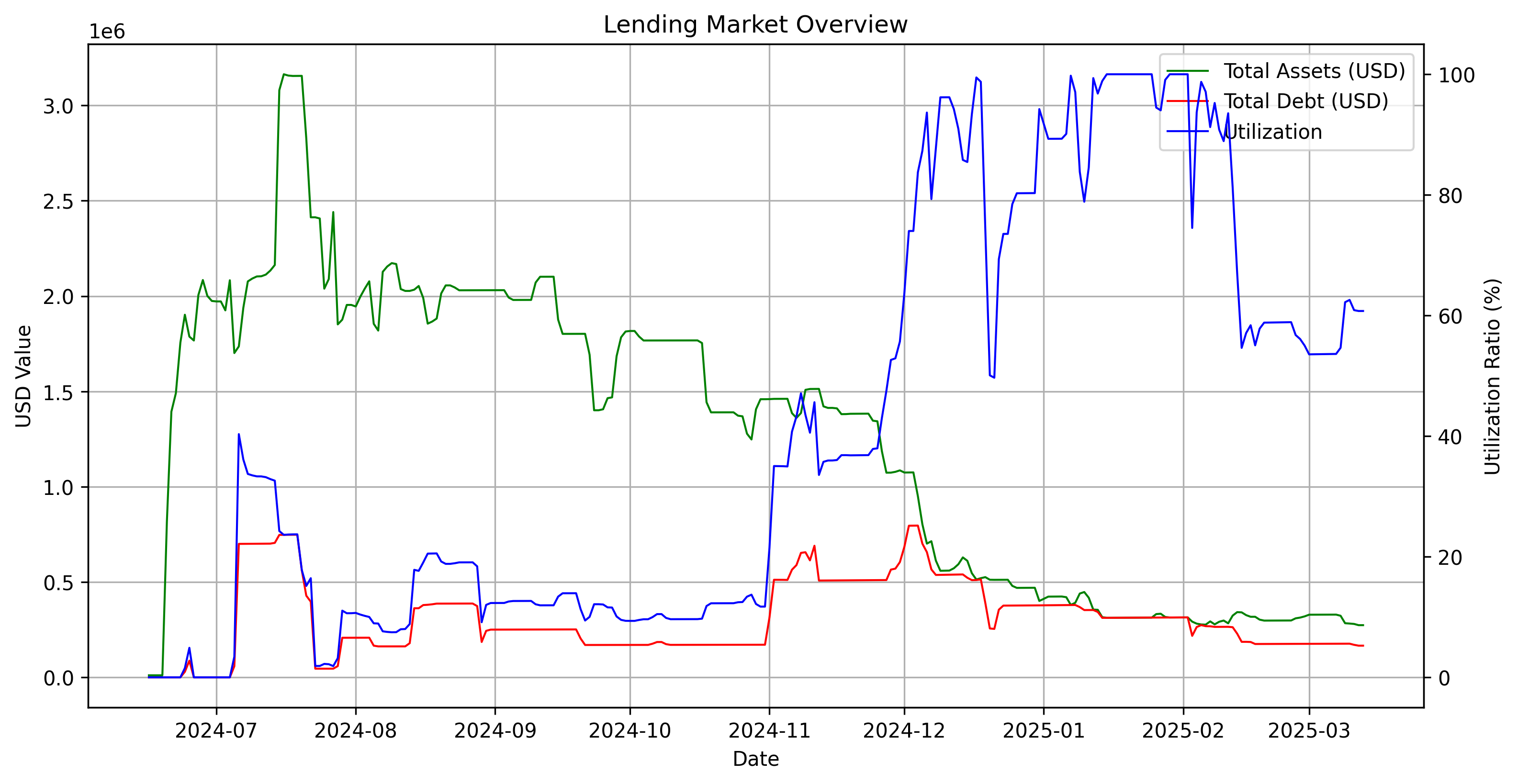
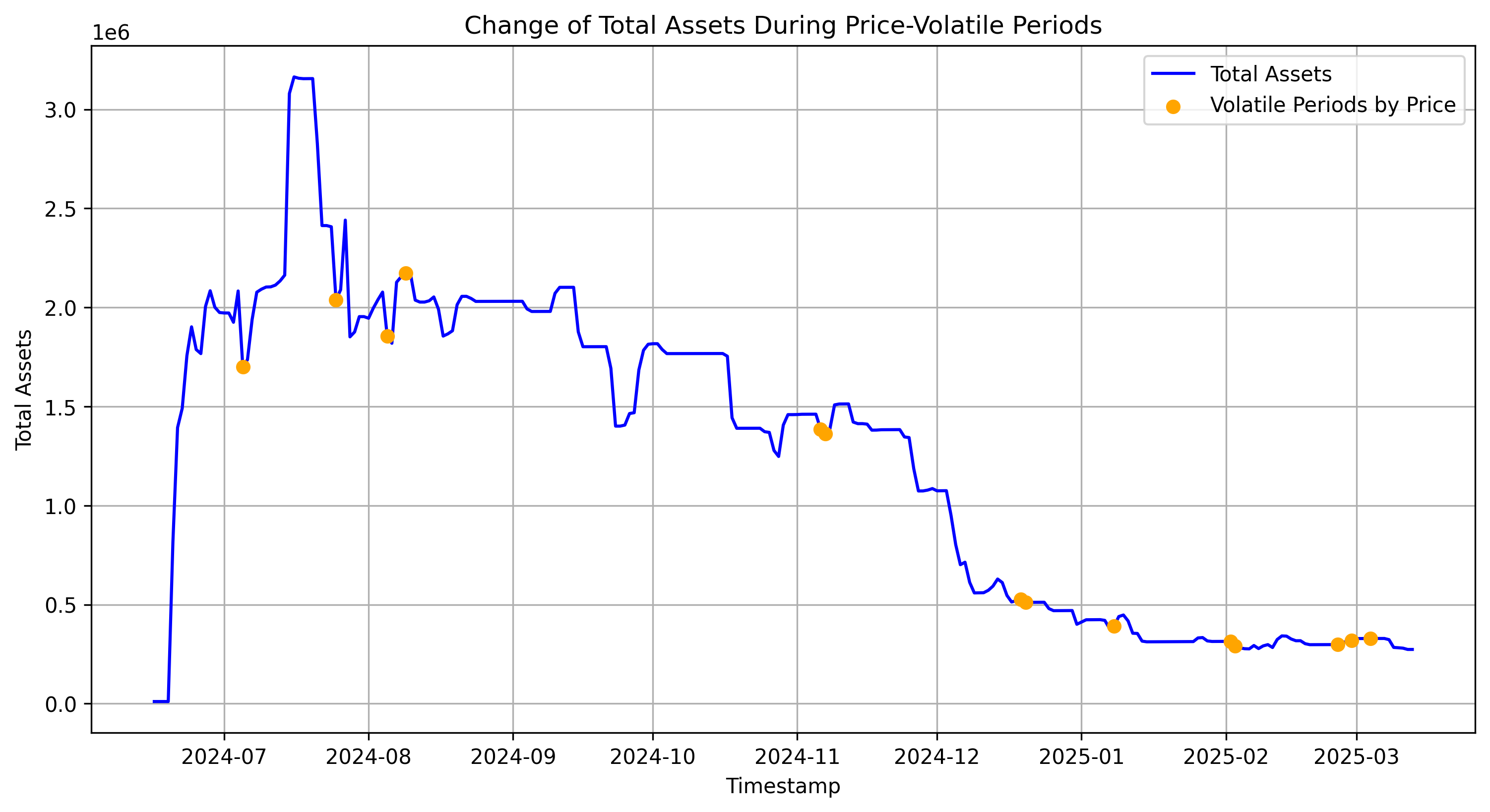
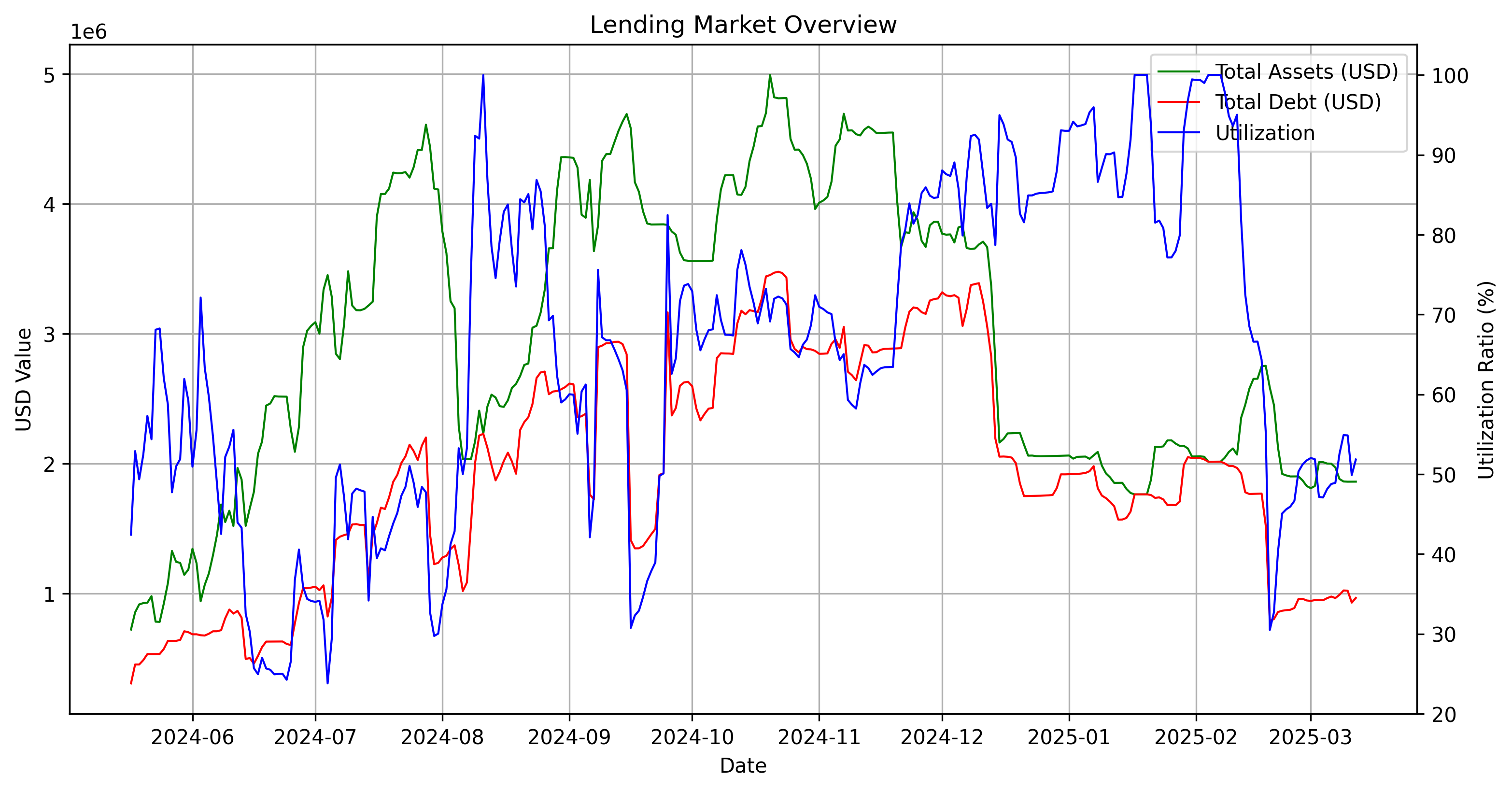
This plot compares total assets and total debt over time while overlaying utilization on a secondary axis.
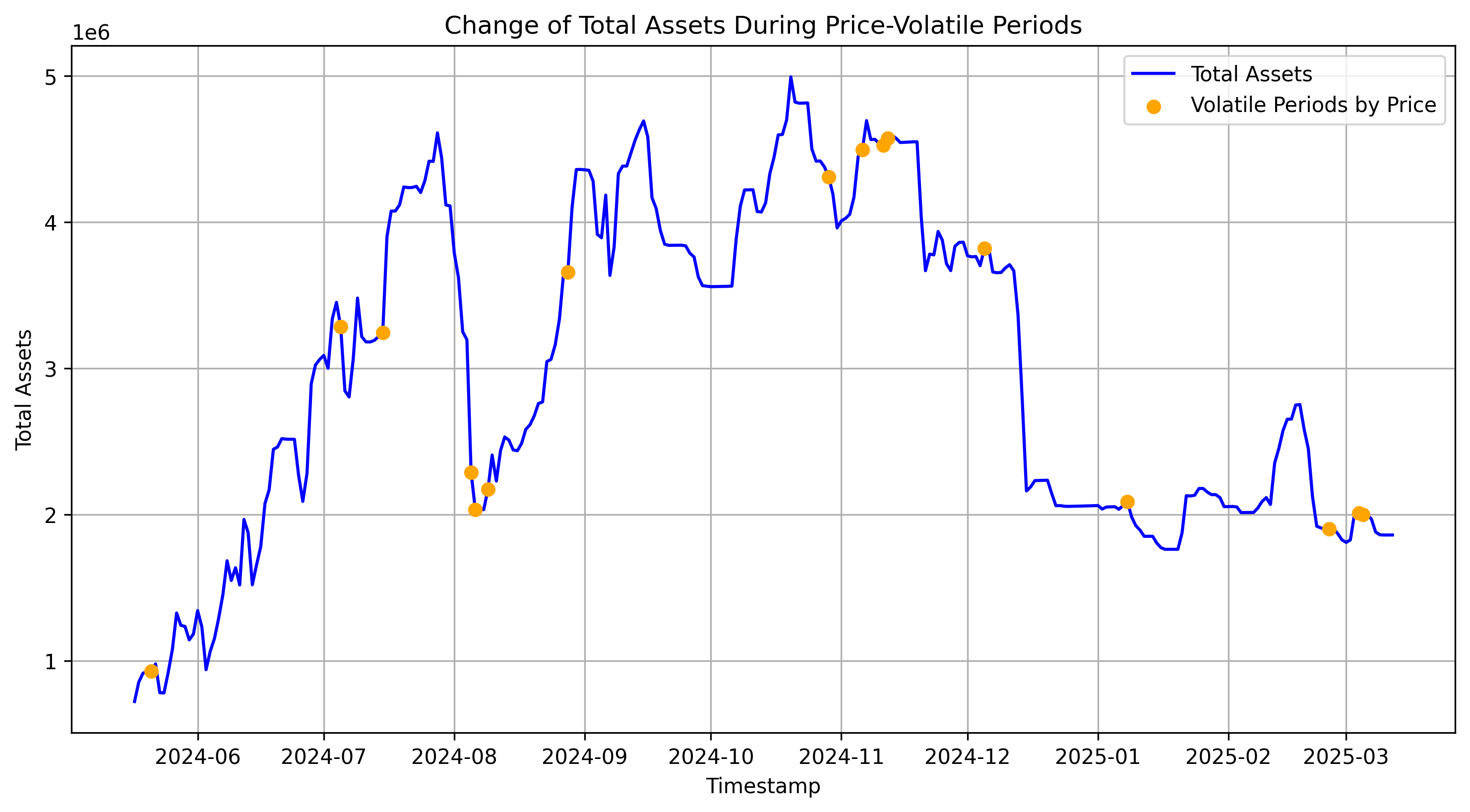
Optimal Utilization Analysis
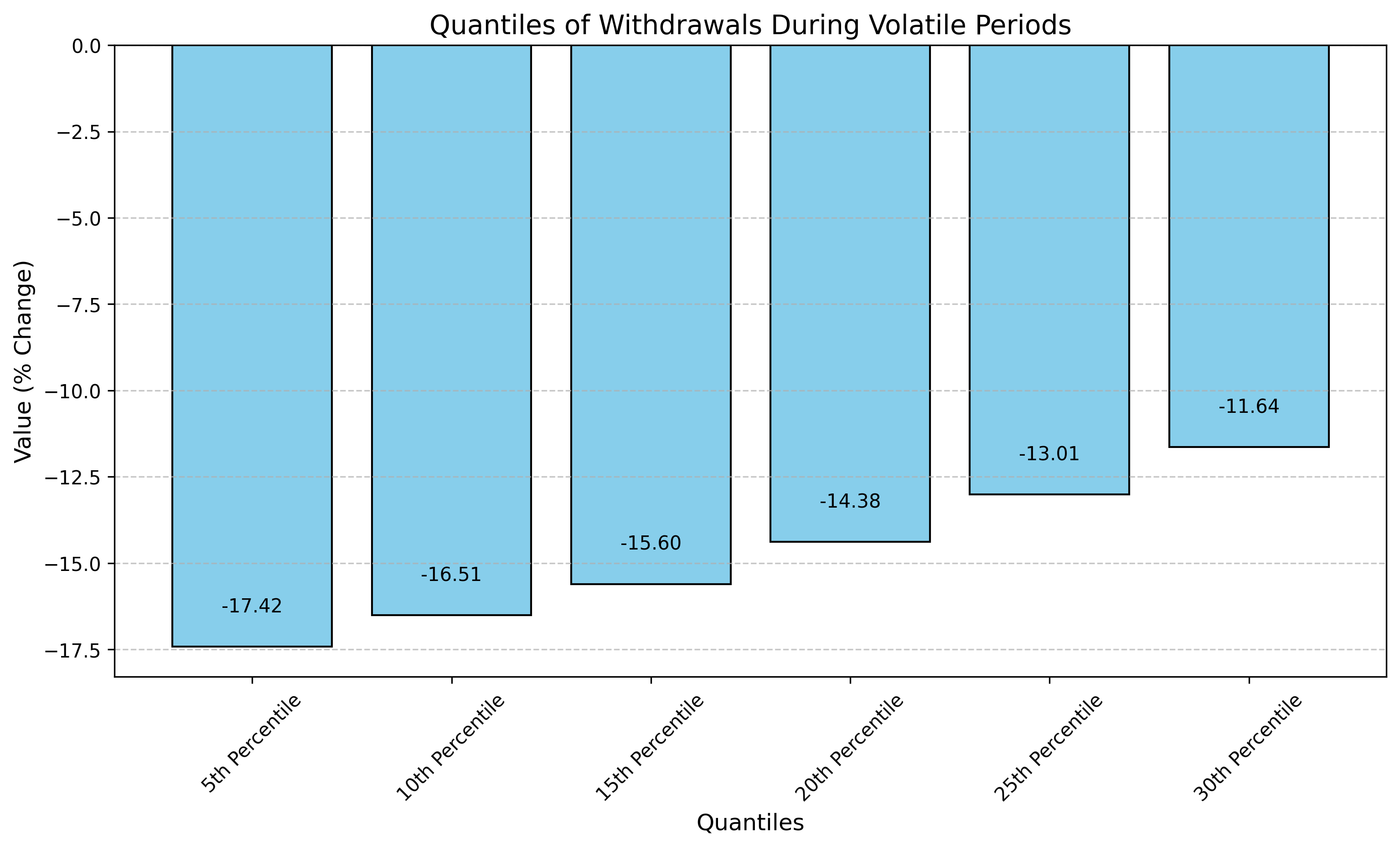
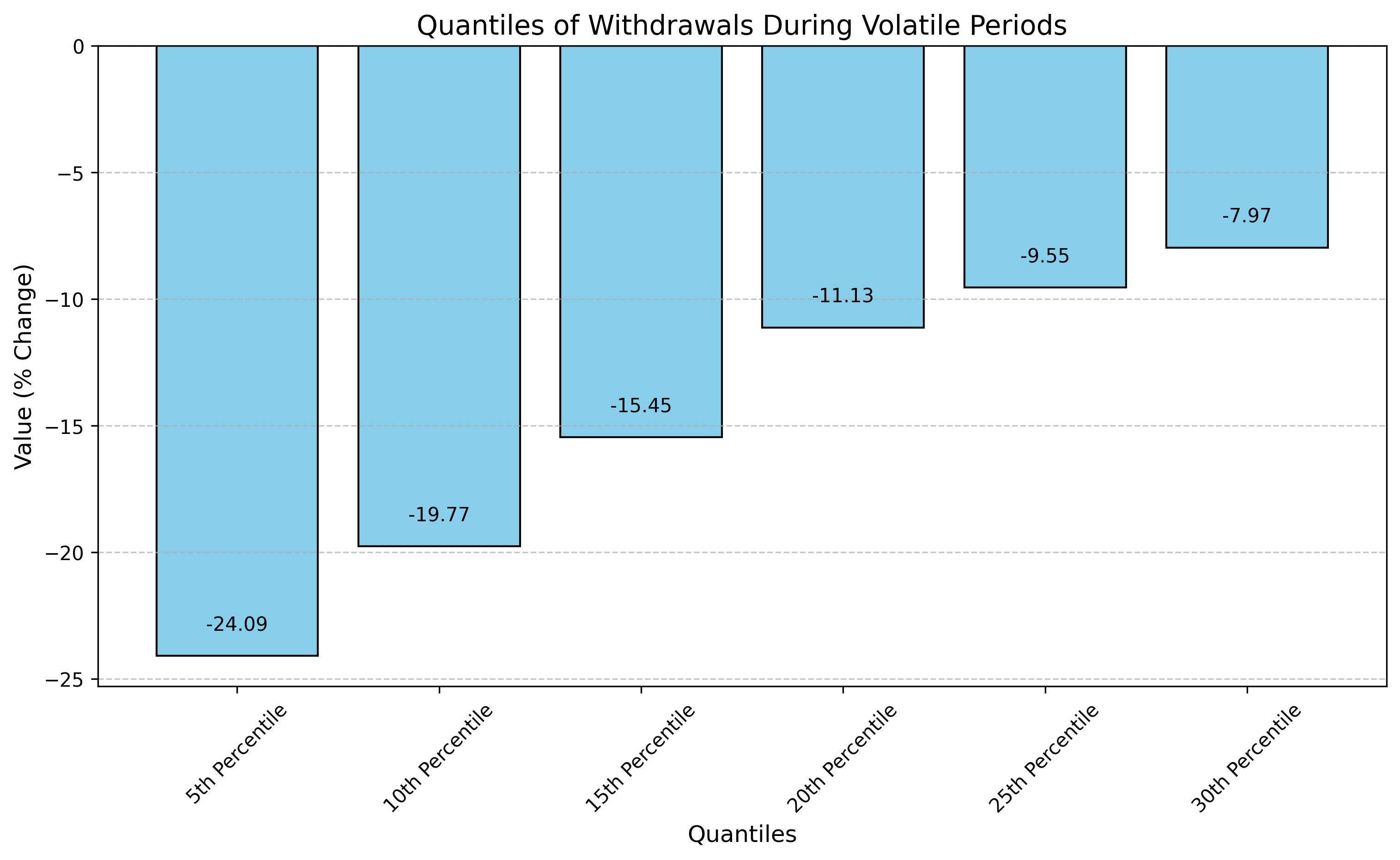
We identify volatile periods based on the price oracle feed and then analyze the withdrawal quantile of total assets during these periods.
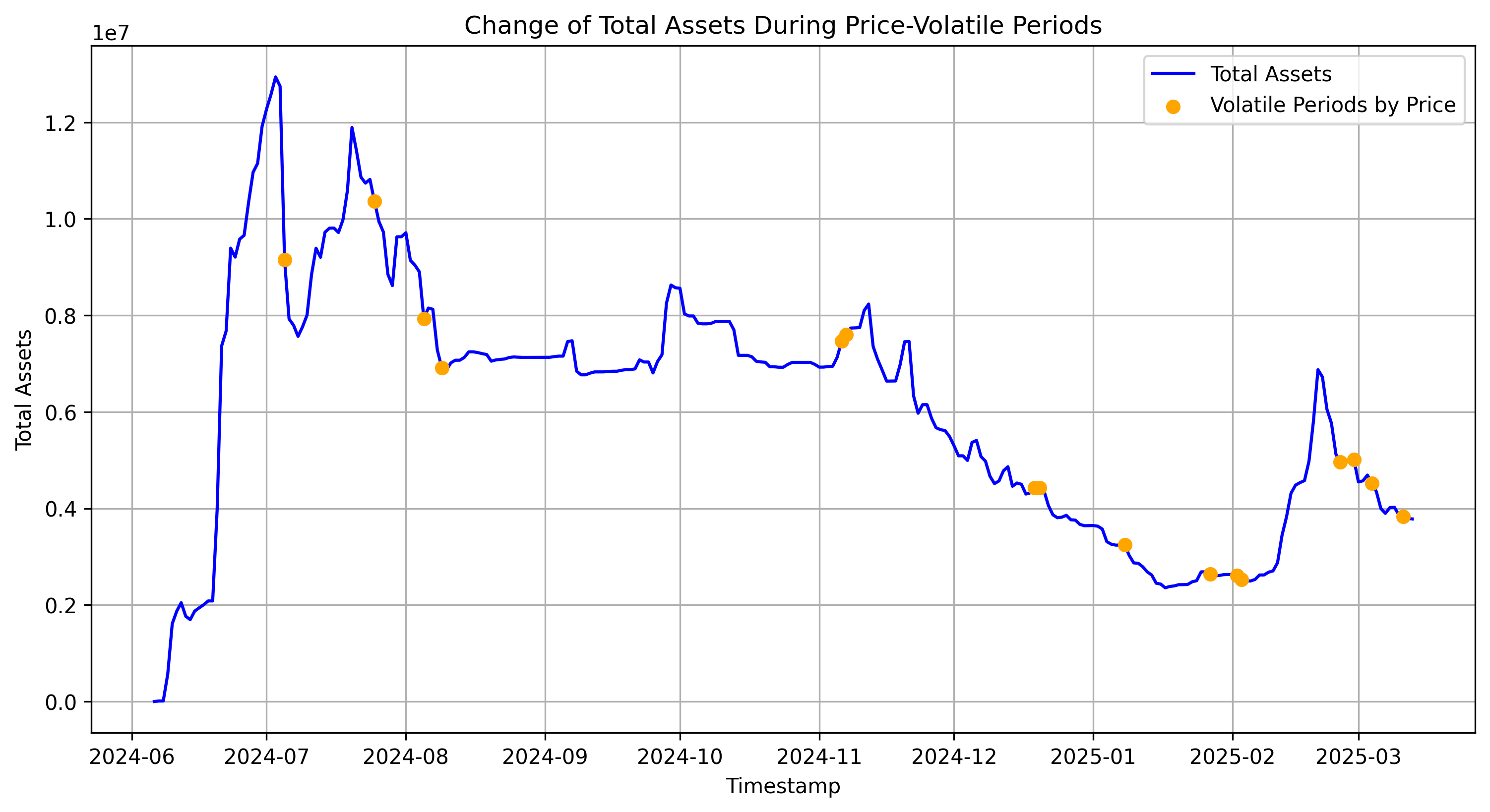
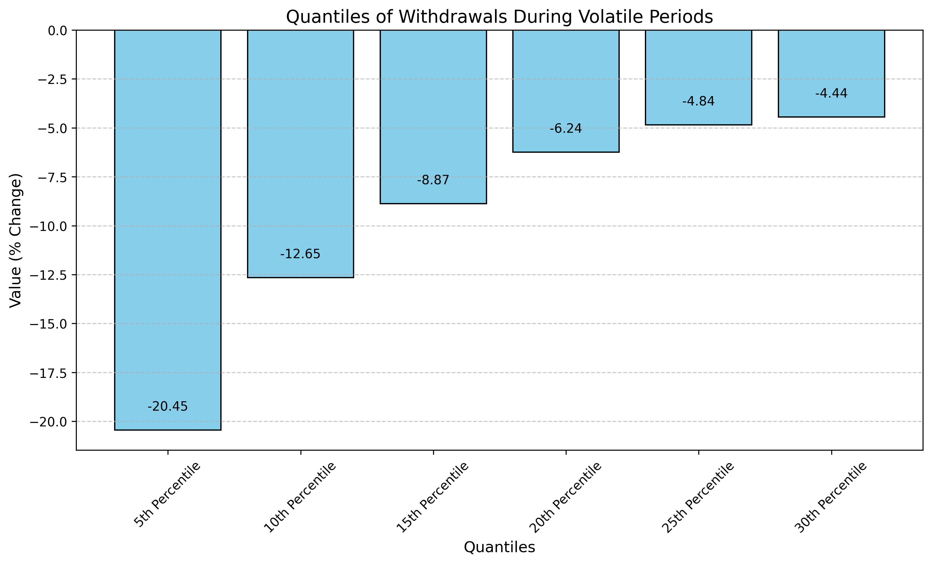
The 10th percentile of negative withdrawals of supplied crvUSD during volatile periods was 13% of the total supply. This means that 90.0% of all observed withdrawals during volatile periods were less than or equal to this value. We define optimal utilization as min(1- withdrawal_quantile, 0.85), so we assign optimal utilization at 85%.
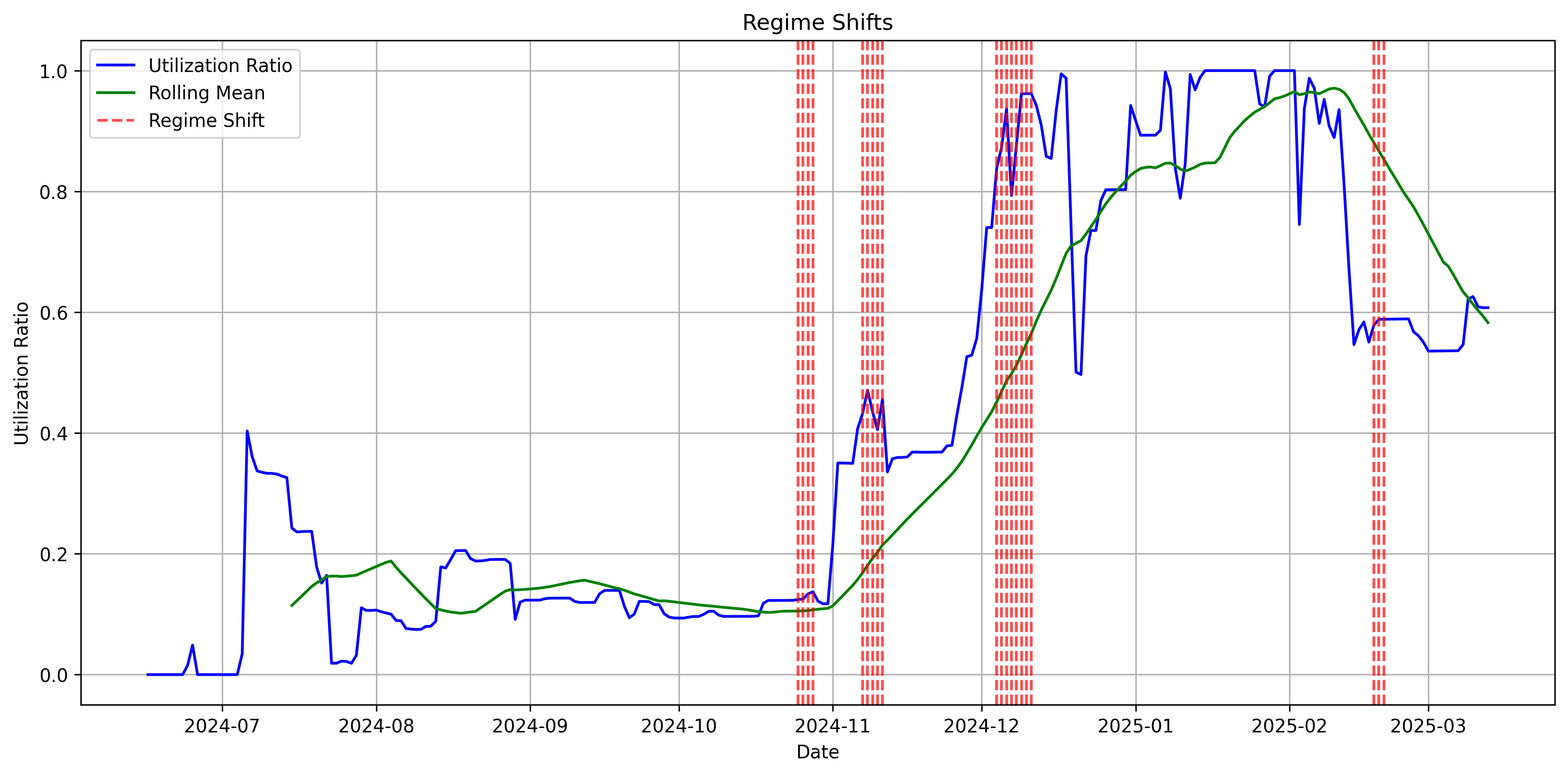
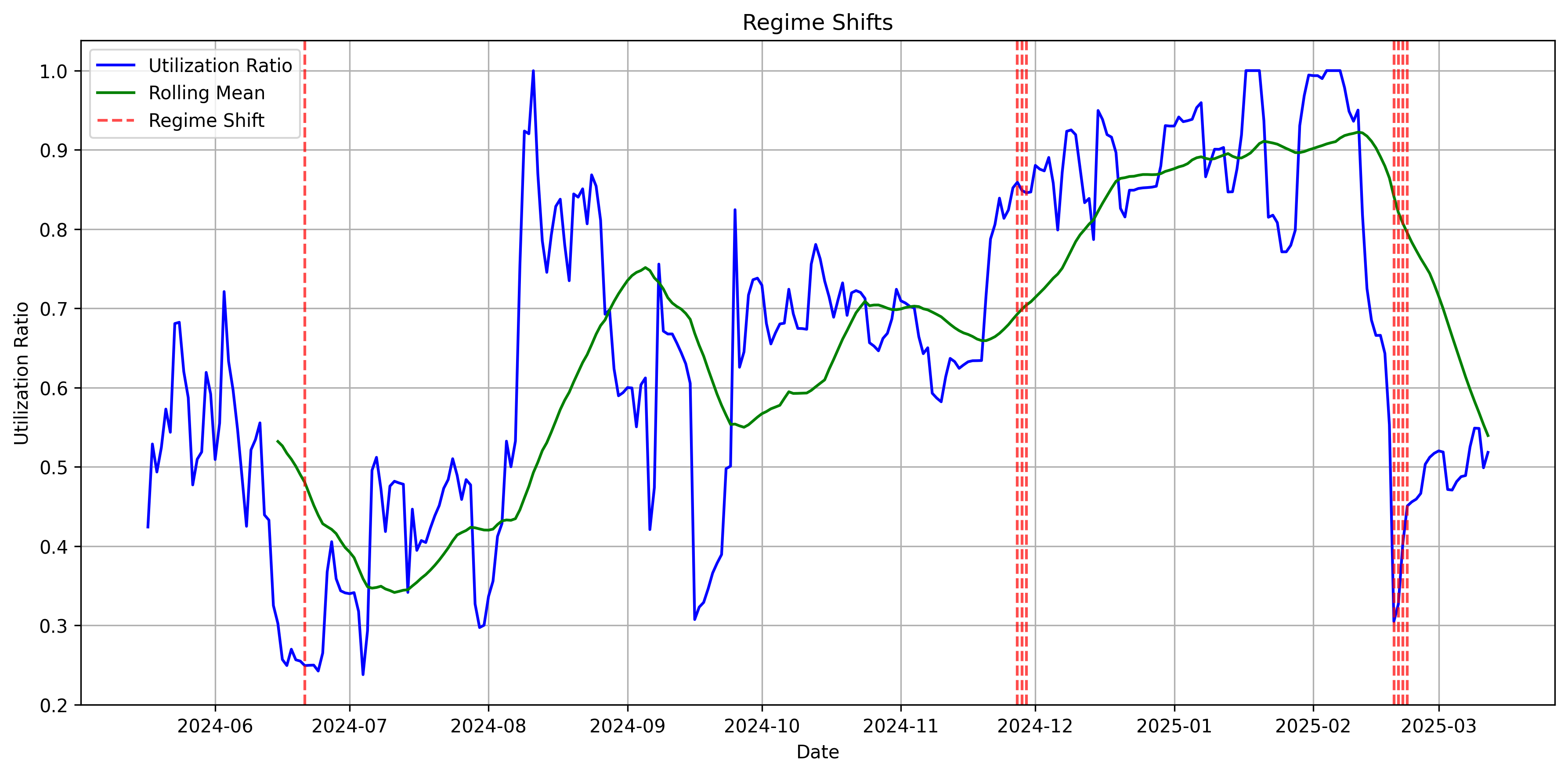
Regime Shift Analysis
This plot shows detected regime shifts in utilization. Red vertical lines indicate significant shifts, which represents changes in stability in utilization in this given market.
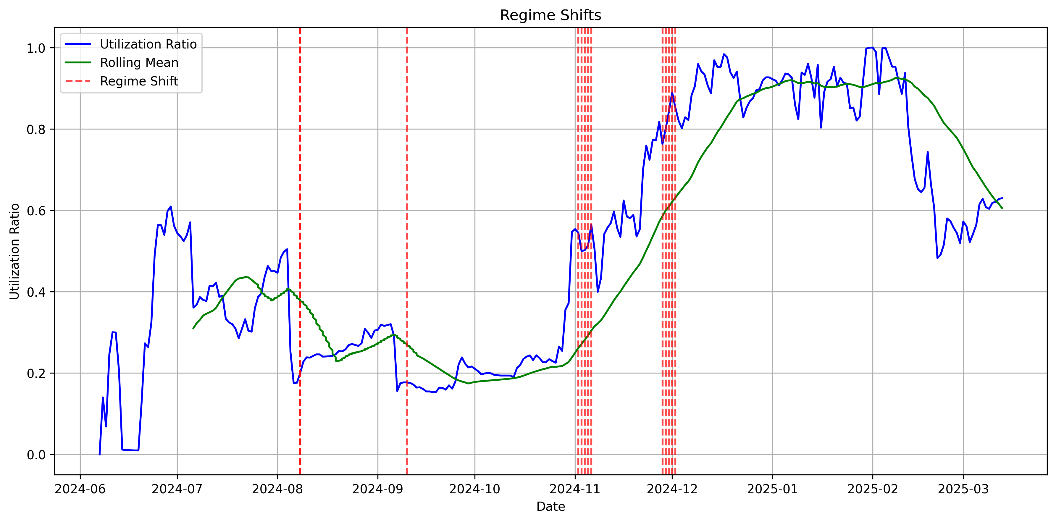
The latest stable regime shift was detected on 2024-12-02.We ended observation on 2025-03-13, covering a period of 101 days.
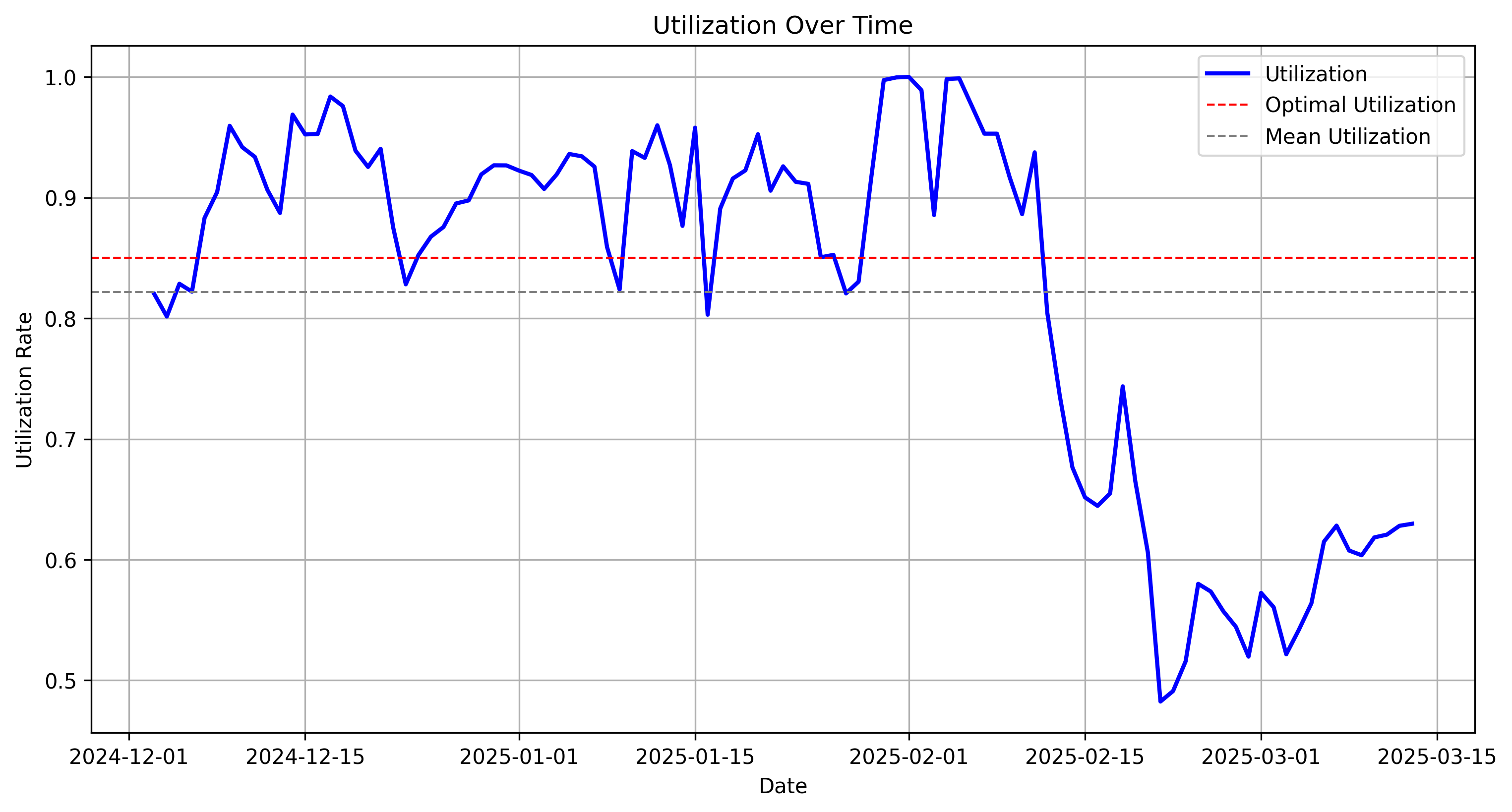
The identified regime can be categorized as slight under our target utilization (82% mean utilization vs 85% target).
Parameterizing of the underlying Model
We estimate the underlying model parameters for the Stochastic differential equation using a simple OLS model.
OLS Regression Results
==============================================================================
Dep. Variable:      delta_utilization   R-squared:                       0.159
Model:                            OLS   Adj. R-squared:                  0.141
Method:                 Least Squares   F-statistic:                     8.613
Date:                Thu, 13 Mar 2025   Prob (F-statistic):           0.000375
Time:                        15:25:56   Log-Likelihood:                 186.69
No. Observations:                  94   AIC:                            -367.4
Df Residuals:                      91   BIC:                            -359.8
Df Model:                           2
Covariance Type:            nonrobust
=========================================================================================
                            coef    std err          t      P>|t|      [0.025      0.975]
-----------------------------------------------------------------------------------------
const                     0.0301      0.008      3.630      0.000       0.014       0.047
borrow_apr_lag           -0.1790      0.046     -3.875      0.000      -0.271      -0.087
delta_utilization_lag     0.1546      0.096      1.615      0.110      -0.036       0.345
==============================================================================
Omnibus:                        5.877   Durbin-Watson:                   1.866
Prob(Omnibus):                  0.053   Jarque-Bera (JB):                5.239
Skew:                           0.495   Prob(JB):                       0.0729
Kurtosis:                       3.599   Cond. No.                         27.9
==============================================================================

Notes:
[1] Standard Errors assume that the covariance matrix of the errors is correctly specified.
⚠️ WARNING: High p-values:
delta_utilization_lag: 0.1099
It important to note the context of this regime and the potential risk of using it to make policy recommendation. Beyond the weak p-values, this market has undergone several major IRM changes, such as reversion from SecondaryMP. We therefore advise caution in implementing the recommended parameters without additional historical data.
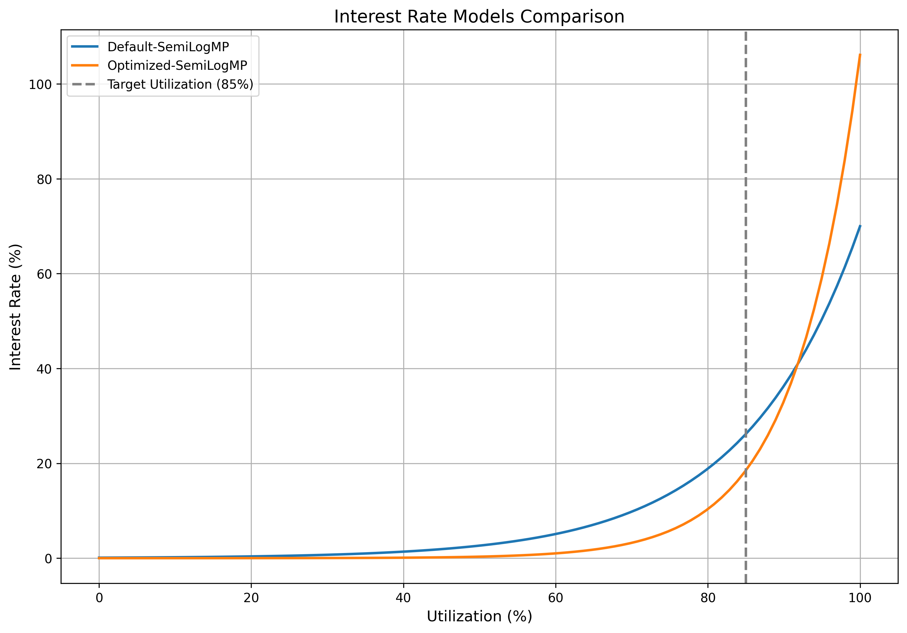
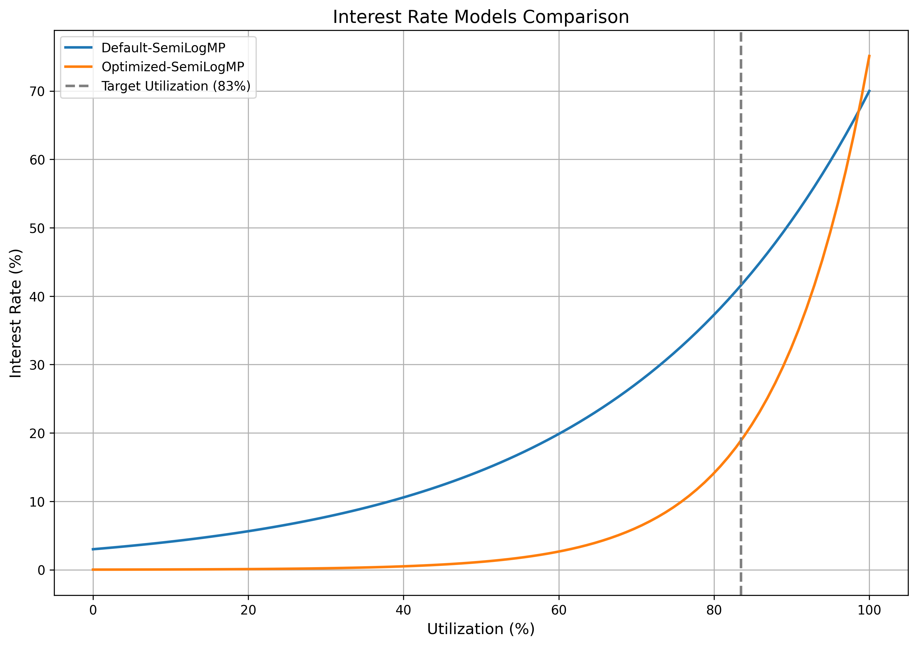
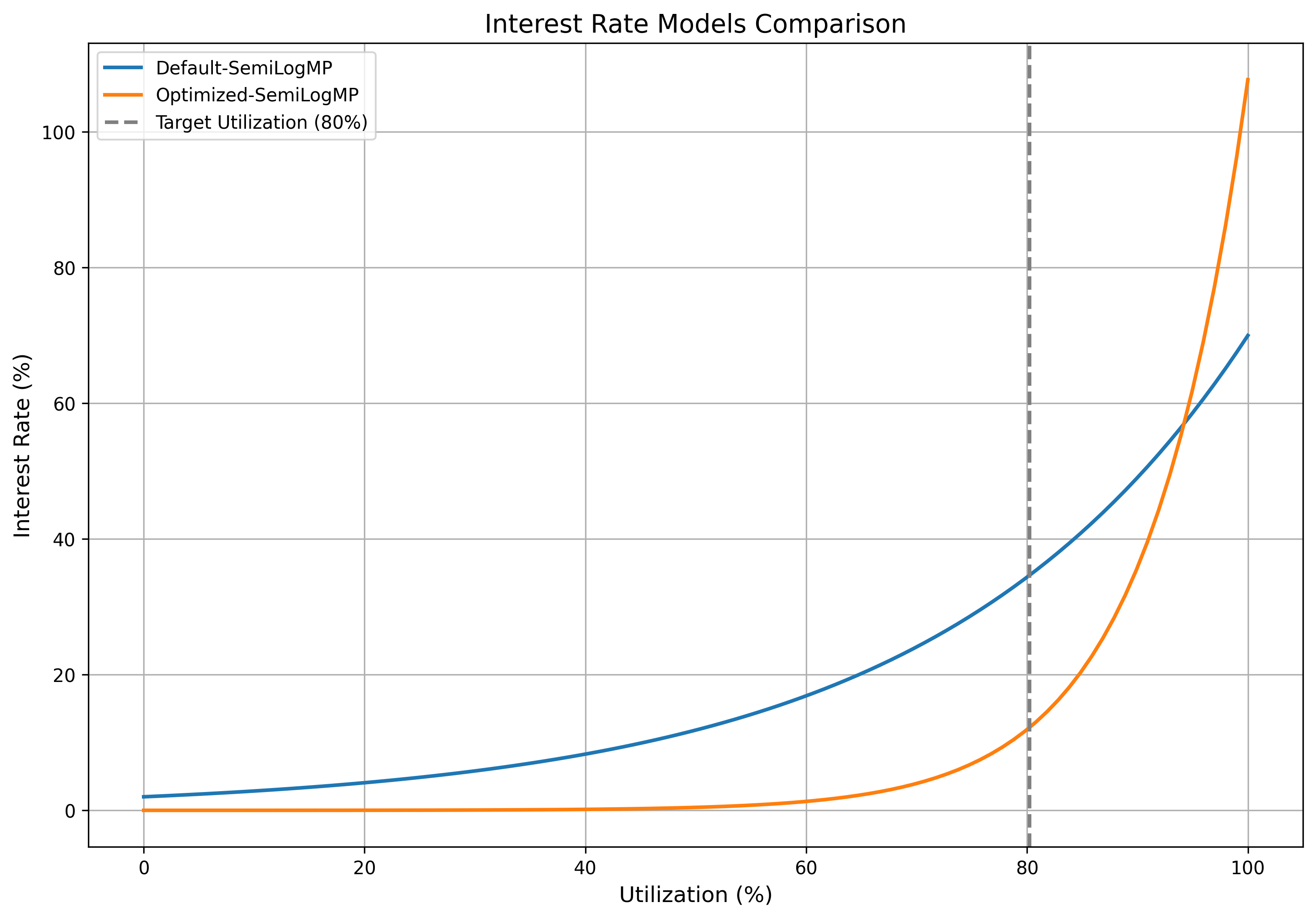
Identifying Optimal Parameters
After optimizing with the composite loss function across multiple simulated SDE paths, we identified the optimal parameters as:
| IRM Label | rate_min | rate_max |
|---|---|---|
Optimized-SemiLogMP |
0.00001 |
1.06136 |
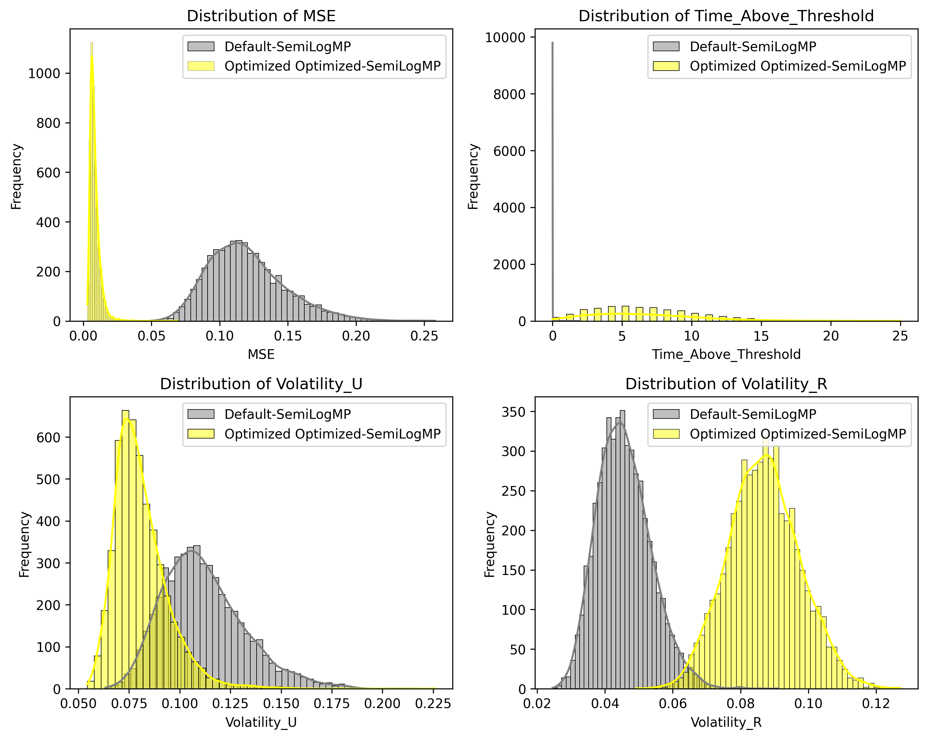
Evaluating Parameter Performance
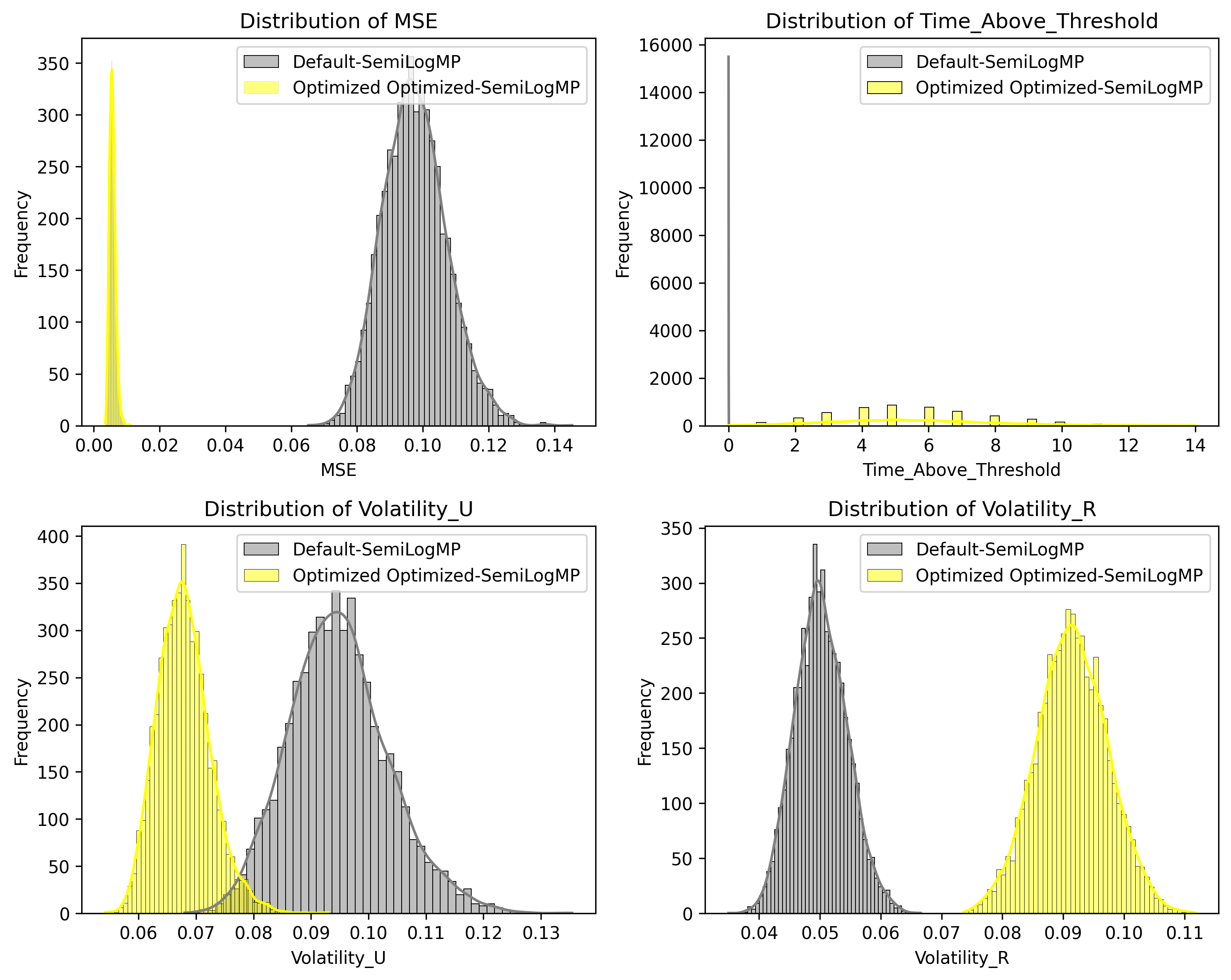
In this section, we compare the default configuration of parameters with the optimized parameters across key performance metrics.
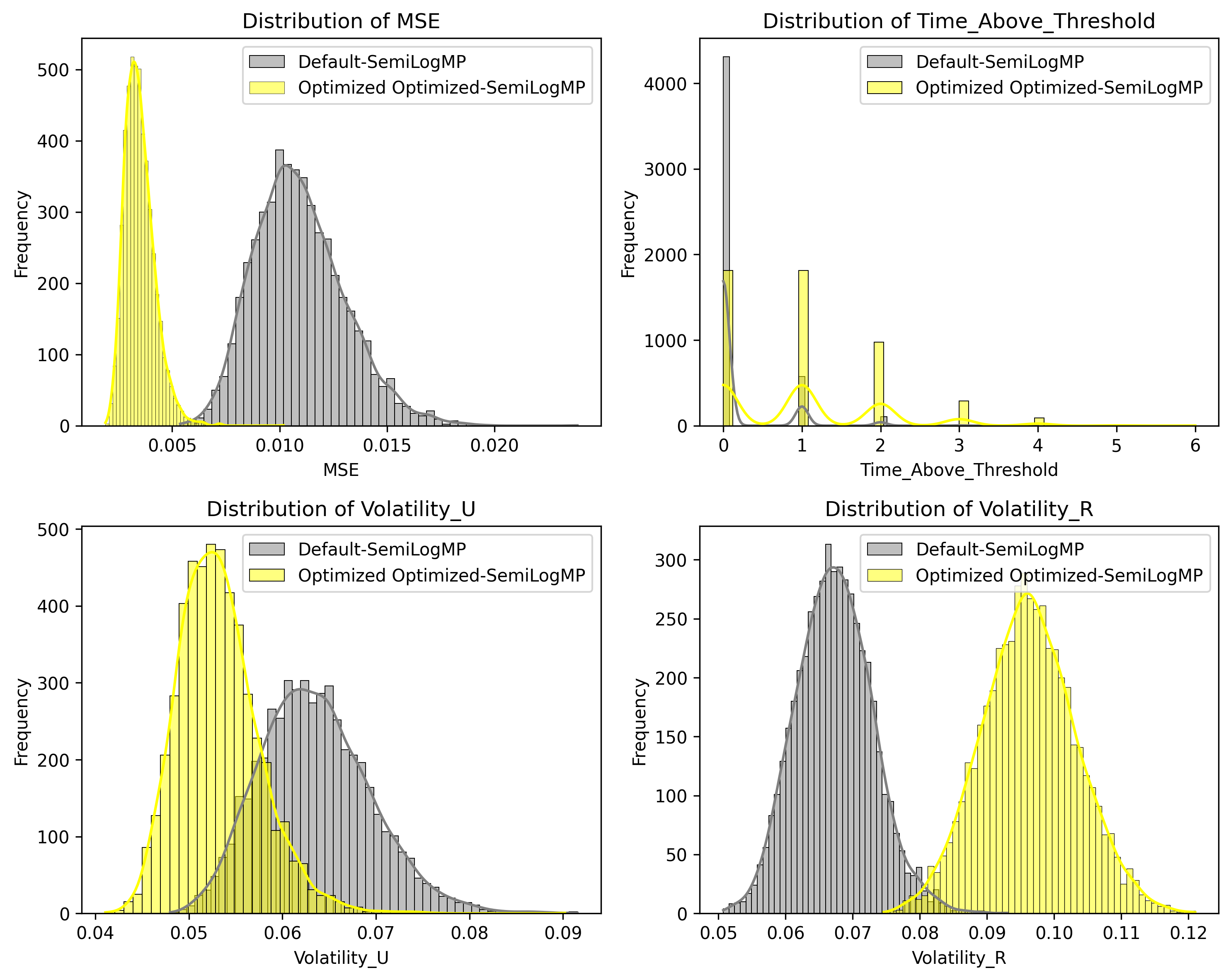
The chart suggests that:
- Mean Squared Error (MSE) is lower for the Optimized Model, hence it trades closer to the optimal utilization level defined.
- Time Above Threshold is higher for the optimized model.
- The Volatility of the Utilization is lower on the Optimized model, suggesting stability in utilization level
- The Volatility of the Rate is higher which marks the fundamental trade-off to manage rates effectively.
Conclusion
The Optimized Model consistently outperforms the default configuration, balancing trade-offs between rate volatility and MSE. However, caution should be exercised in implementing this configuration due to the changes in IRM policy that occurred over the sample period.
wstETH-long2 Analysis
wstETH-long2
The wstETH-long2 market is deployed on Ethereum with the controller address:0x5756A035F276a8095A922931F224F4ed06149608.
The current Interest Rate Model (IRM) is SemiLogIRM, with the following parameters:
-
min_rate= 0.005 -
max_rate= 0.7
This plot compares total assets and total debt over time while overlaying utilization on a secondary axis.
Optimal Utilization Analysis
We identify volatile periods based on the price oracle feed and then analyze the withdrawal quantile of total assets during these periods.
The 10th percentile of negative withdrawals of supplied crvUSD during volatile periods was 17% of the total supply.This means that 90.0% of all observed withdrawals during volatile periods were less than or equal to this value. Given that optimal utilization is defined as min(1- withdrawal_quantile, 0.85), optimal utilization is 83%.
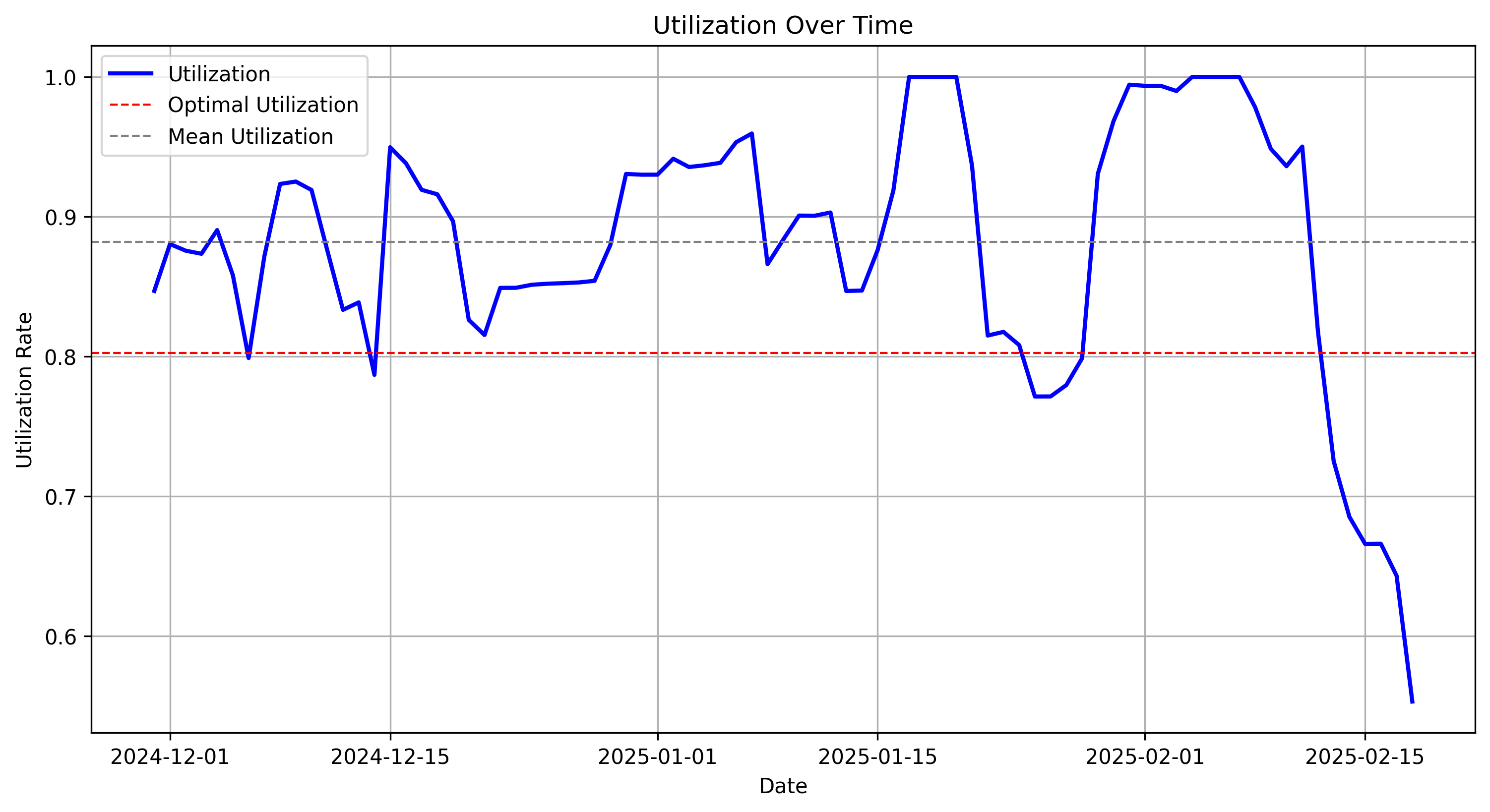
Regime Shift Analysis
This plot shows detected regime shifts in utilization. Red vertical lines indicate significant shifts, which represents changes in utilization stability in this given market.
The latest stable regime shift was detected on 2024-12-11. We ended observation on 2025-02-18, covering a period of 69 days.
The regime is characterized by over-utilization, with the mean utilization (88%) higher than the recommended utilization target (83%).
Parameterizing of the underlying Model
We estimate underlying model parameters for the Stochastic differential equation using a simple OLS model.
OLS Regression Results
==============================================================================
Dep. Variable:      delta_utilization   R-squared:                       0.248
Model:                            OLS   Adj. R-squared:                  0.222
Method:                 Least Squares   F-statistic:                     9.706
Date:                Thu, 13 Mar 2025   Prob (F-statistic):           0.000227
Time:                        16:40:47   Log-Likelihood:                 104.50
No. Observations:                  62   AIC:                            -203.0
Df Residuals:                      59   BIC:                            -196.6
Df Model:                           2
Covariance Type:            nonrobust
=========================================================================================
                            coef    std err          t      P>|t|      [0.025      0.975]
-----------------------------------------------------------------------------------------
const                     0.0539      0.015      3.590      0.001       0.024       0.084
borrow_apr_lag           -0.3163      0.080     -3.936      0.000      -0.477      -0.155
delta_utilization_lag     0.2588      0.114      2.280      0.026       0.032       0.486
==============================================================================
Omnibus:                        6.883   Durbin-Watson:                   1.913
Prob(Omnibus):                  0.032   Jarque-Bera (JB):                6.532
Skew:                           0.559   Prob(JB):                       0.0382
Kurtosis:                       4.131   Cond. No.                         19.8
==============================================================================

Notes:
[1] Standard Errors assume that the covariance matrix of the errors is correctly specified.
It’s important to note the context of this regime and the potential risk of using it to make policy recommendation. Beyond the weak p-values, this market has undergone several major IRM changes, such as reversion from SecondaryMP. We, therefore, advise great caution implementing these parameter recommendations without additional data.
Identifying Optimal Parameters
After optimizing with the composite loss function across multiple simulated SDE paths, we identified the optimal parameters as:
| IRM Label | rate_min | rate_max |
|---|---|---|
Optimized-SemiLogMP |
0.00018 |
0.75117 |
Evaluating Parameter Performance
The chart suggests that:
- Mean Squared Error (MSE) is lower for the Optimized Model, hence it trades closer to the optimal utilization level defined.
- Time Above Threshold is higher for the optimized model, meaning the market will likely operate above the target utilization more often than in the current configuration.
- The Volatility of the Utilization is lower on the Optimized model suggesting stability in utilization level
- The Volatility of the Rate is higher which marks the fundamental trade-off to manage rates effectively.
Conclusion
The Optimized Model consistently outperforms the default configuration. It is apparent that the model tolerates more rate flexibility with an exaggerated IRM curvature. This may the reason why, despite overutilization, a lower rate is suggest at the equilibirum level. Note that the simulation results should be enjoyed with caution due the multiple changes in this regime that may have biased the underlying model.
WBTC-long Analysis
WBTC-long
The WBTC-long market is deployed on Ethereum with the controller address:0xcaD85b7fe52B1939DCEebEe9bCf0b2a5Aa0cE617.
The current Interest Rate Model (IRM) is SemiLogIRM, with the following parameters:
-
min_rate= 0.005 -
max_rate= 0.7
This plot compares total assets and total debt over time while overlaying utilization on a secondary axis.
Optimal Utilization Analysis
We identify volatile periods based on the price oracle feed and then analyze the withdrawal quantile of total assets during these periods.
The 10th percentile of negative withdrawals of supplied crvUSD during volatile periods was 20% of the total supply.This means that 90% of all observed withdrawals during volatile periods were less than or equal to this value. Given that optimal utilization is defined as min(1- withdrawal_quantile, 0.85), optimal utilization is 80%.
Regime Shift Analysis
This plot shows detected regime shifts in utilization. Red vertical lines indicate significant shifts, which represents changes in utilization stability in this given market.
The last stable regime shift was detected on 2024-11-29. We ended observation on 2025-02-19, covering a period of 82 days.
The regime is characterized by over-utilization, with a mean utilization of 88% compared to a recommended target utilization of 80%.
Parameterizing of the underlying Model
We estimate the underlying model parameters for the Stochastic differential equation using a simple OLS model.
OLS Regression Results
==============================================================================
Dep. Variable:      delta_utilization   R-squared:                       0.121
Model:                            OLS   Adj. R-squared:                  0.096
Method:                 Least Squares   F-statistic:                     4.895
Date:                Thu, 13 Mar 2025   Prob (F-statistic):             0.0102
Time:                        16:48:14   Log-Likelihood:                 160.56
No. Observations:                  74   AIC:                            -315.1
Df Residuals:                      71   BIC:                            -308.2
Df Model:                           2
Covariance Type:            nonrobust
=========================================================================================
                            coef    std err          t      P>|t|      [0.025      0.975]
-----------------------------------------------------------------------------------------
const                     0.0112      0.007      1.519      0.133      -0.003       0.026
borrow_apr_lag           -0.0954      0.049     -1.966      0.053      -0.192       0.001
delta_utilization_lag     0.2608      0.120      2.180      0.033       0.022       0.499
==============================================================================
Omnibus:                        6.214   Durbin-Watson:                   1.782
Prob(Omnibus):                  0.045   Jarque-Bera (JB):                9.467
Skew:                          -0.159   Prob(JB):                      0.00879
Kurtosis:                       4.723   Cond. No.                         36.9
==============================================================================

Notes:
[1] Standard Errors assume that the covariance matrix of the errors is correctly specified.
⚠️ WARNING: High p-values:
const: 0.1331
borrow_apr_lag: 0.0532
It is important to note the context of this regime and the potential risk of using it to make policy recommendation. Beyond the weak p-values, this market has undergone several major IRM changes, such as reversion from SecondaryMP. We, therefore, advise caution when implementing these parameters without additional data.
Identifying Optimal Parameters
After optimizing with the composite loss function across multiple simulated SDE paths, we identified the optimal parameters as:
| IRM Label | rate_min | rate_max |
|---|---|---|
Optimized-SemiLogMP |
0.00002 |
1.07709 |
Evaluating Parameter Performance
In this section, we compare the default configuration of parameters with the optimized parameters across key performance metrics.
The chart suggests that:
- Mean Squared Error (MSE) is lower for the Optimized Model, hence it trades closer to the optimal utilization level defined.
- Time Above Threshold is higher for the optimized model, meaning the optimized market is more likely to operate above target utilization than the current configuration.
- The Volatility of the Utilization is lower on the Optimized model suggesting stability in utilization level
- The Volatility of the Rate is higher which marks the fundamental trade-off to manage rates effectively.
Conclusion
The Optimized Model consistently outperforms the default configuration. It is apparent that the model tolerates more rate flexibility with exaggerated IRM curvature. This may the reason why, despite overutilization, a lower rate is suggested at the target utilization. Note that the simulation results should be enjoyed with caution due the multiple changes in this regime that may have biased the underlying model.
Specification:
ACTIONS = [
    # WETH2 min_rate 0.1%
    ("0x20a32CC24247fBAb1eC3c92a343D5787406BCbf9", "set_rates", 31709791, 22196854388),

    # WBTC min_rate 0.1%
    ("0xE53C7e8857fAd35dF5a02a2899CaF5871A50bA95", "set_rates", 31709791, 22196854388),

    # wstETH2 min_rate 0.2%
    ("0xc246Ee163DFC8Eb599542a915074549A66b216F6", "set_rates", 63419583, 22196854388),

]