Replace sUSDe-long-v2 LlamaLend SecondaryMP with Semilog

Summary

Set the sUSDe-long-v2 LlamaLend monetary policy to Semilog deployed here with min/max params set to 0.004% / 47.658%.

Motivation

  • Secondary Monetary Policy imposes artificial rate caps, limiting effective risk management by introducing an external dependency to assign market rates.
  • High interest rates serve as vital signals, reflecting actual market risk and promoting system stability.
  • A Semilog IRM allows responsive, dynamic interest rate adjustments, effectively discouraging excessive borrowing during market stress and encouraging timely repayments.
  • Market-driven dynamics will naturally regulate interest rates, promoting sustainable performance based on conditions internal to the lend market.

The current SecondaryMP interest rate model for sUSDe is pegged externally to the sUSDe APR, thus imposing a rigid ceiling on maximum LlamaLend interest rates based on sUSDe revenue distribution. While intended to regulate borrowing costs with respect to the sUSDe yield trends, this model increases systemic risks for LlamaLend, exposing it to additional external dependencies.

Enhancing Risk Mitigation: Prioritizing Lenders

LlamaLend must prioritize lender protection to minimize the risk of accruing bad debt. Persistent maximum utilization (such as seen in the past in former SecondaryMP Market) often signals systemic distress.

Under current SecondaryMP conditions, artificially capped APRs limit the protocol’s ability to discourage borrowing and stimulate repayments effectively, exacerbating potential illiquidity and bad debts if underlying assets depreciate. For instance, if sUSDe experiences significant volatility or begins to depeg, borrowers could exploit the artificially limited APR by maximizing borrowing, liquidating collateral such as crvUSD, and abandoning positions.

By contrast, SemilogMP assigns rates purely according to the LlamaLend market’s utilization and min/max bounds assigned by DAO governance. This offers the Curve DAO more direct control over supply/demand regulation. Eliminating external rate referencing enables organic market self-correction through inherent supply and demand mechanisms, minimizing vulnerability to exploitation and unforeseen systemic risks. Given this, we advocate for the sUSDe transition to a Semilog Interest Rate Model.

sUSDe Semilog Model Parameterization Analysis

To accurately identify safe and effective market-driven interest rates, we employed our simulation framework for IRM parameter optimization.

Detailed methodology: LlamaLend Monetary Policy Optimization

sUSDe-long IRM Analysis and Results

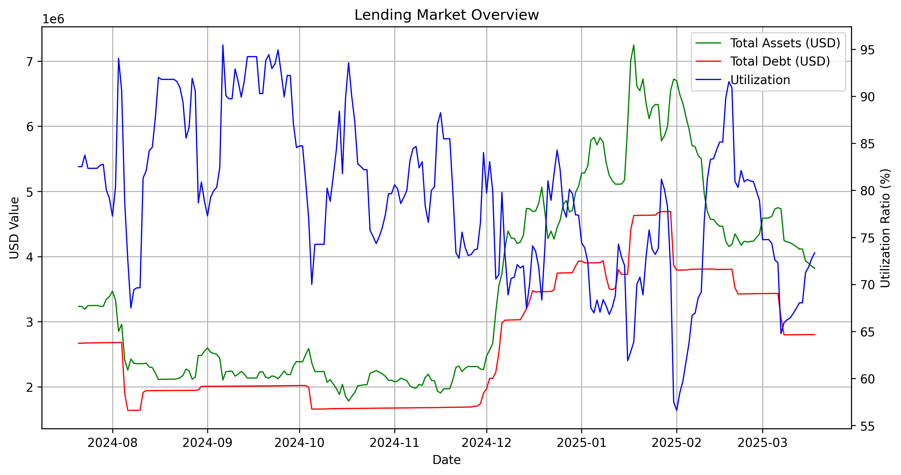
sUSDe-long-v2 is currently deployed on Ethereum with controller address: 0xB536FEa3a01c95Dd09932440eC802A75410139D6. The current IRM is a SecondaryMP model referencing sUSDe yield externally.

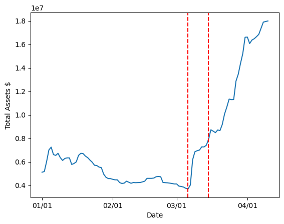
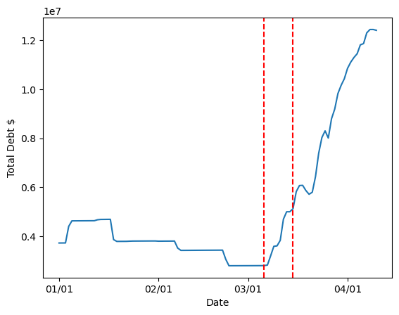
The following plot illustrates total assets, total debt, and utilization over time:

Optimal Utilization Analysis

First we determine a target utilization for the market according to historical market data. We analyzed volatile periods, identified through the oracle price feed, and measured asset withdrawal behavior during volatile periods:

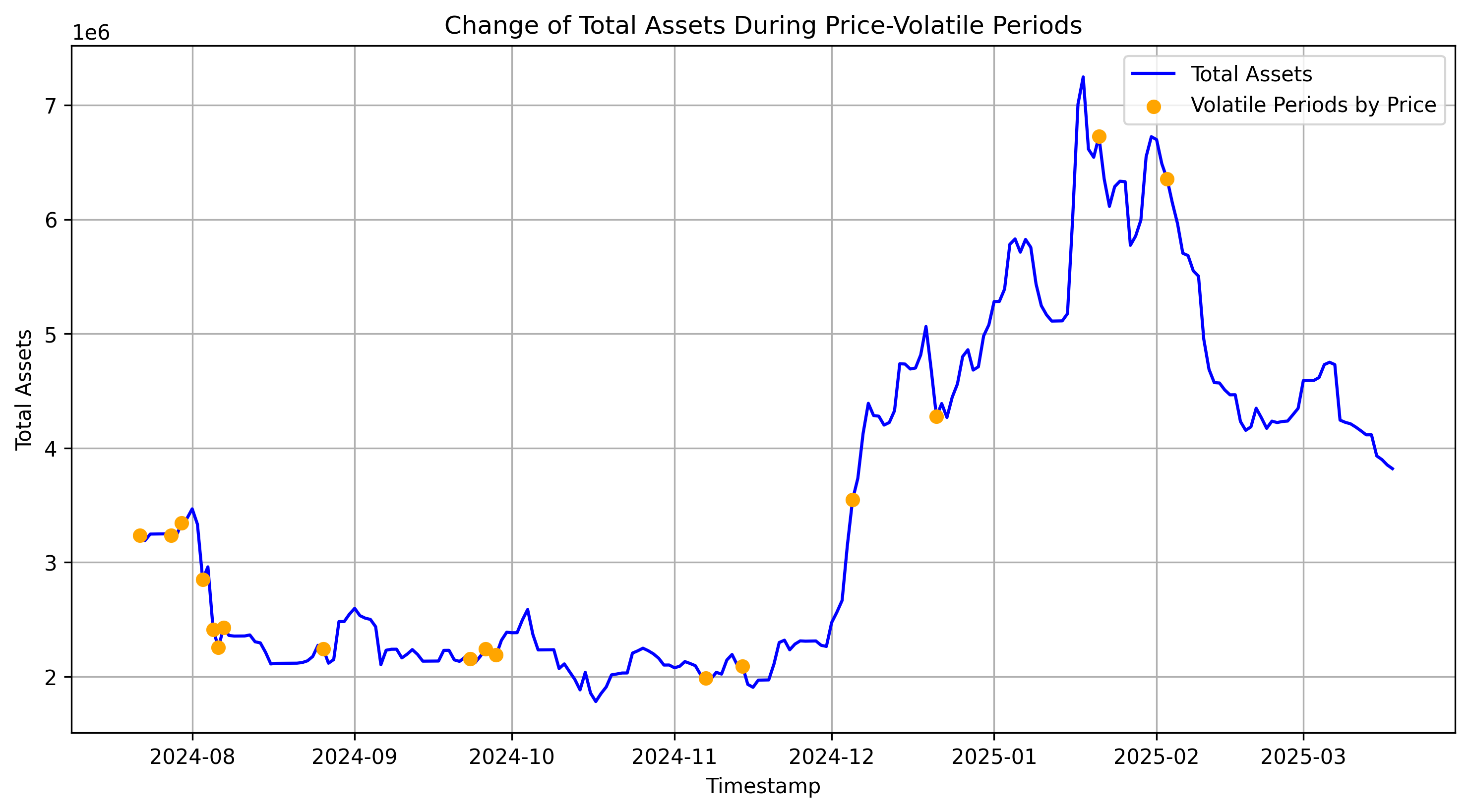
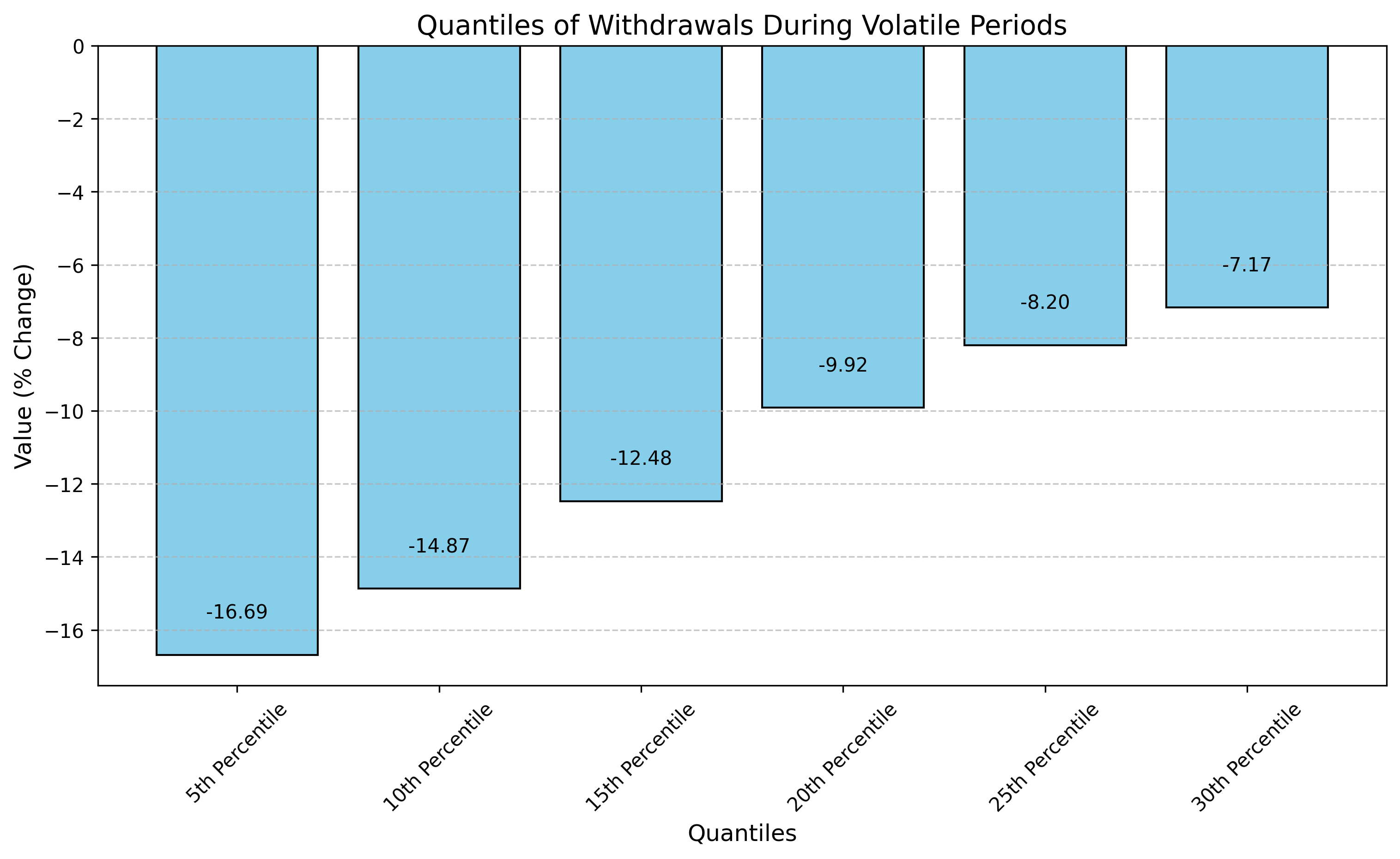
During volatility, the 10th percentile of negative withdrawals of supplied crvUSD was 85%, indicating 90% of withdrawals stayed within this bound. Thus, optimal utilization is conservatively set at 85%, calculated as min(1 - withdrawal_quantile, 0.85).

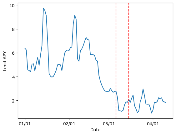
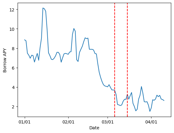
Regime Shift Detection

Significant regime shifts in utilization dynamics (marked by red vertical lines below) indicate changes in market stability, indicating thresholds when the market may require reparameterization:

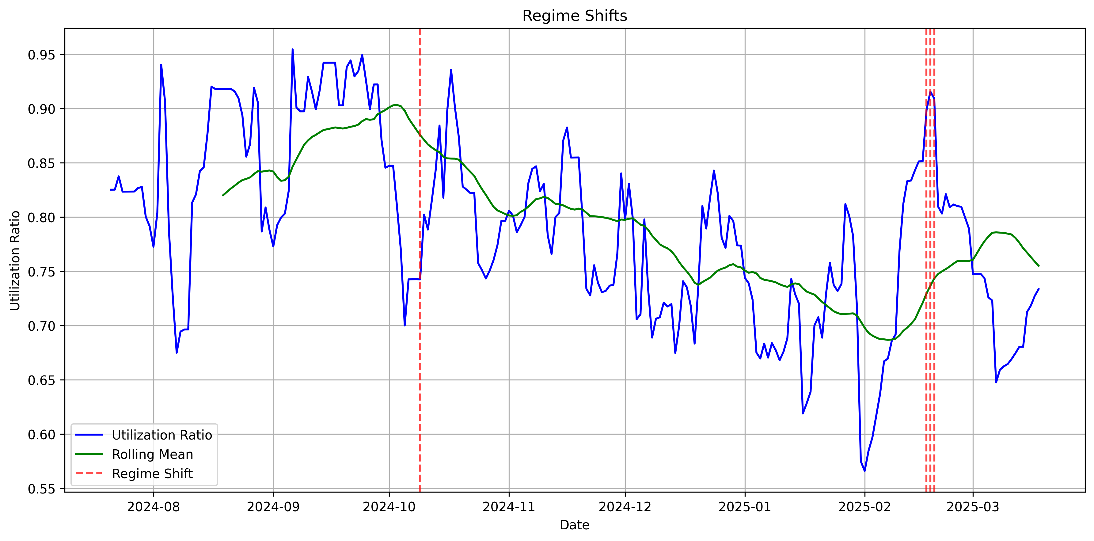
The last stable regime shift was observed on 2024-10-09. Our analysis spans until 2025-02-17 (131 days), excluding the latest period due to insufficient data for reliable parameter estimation.

Below, we compare empirical utilization against the optimal target within the selected regime:

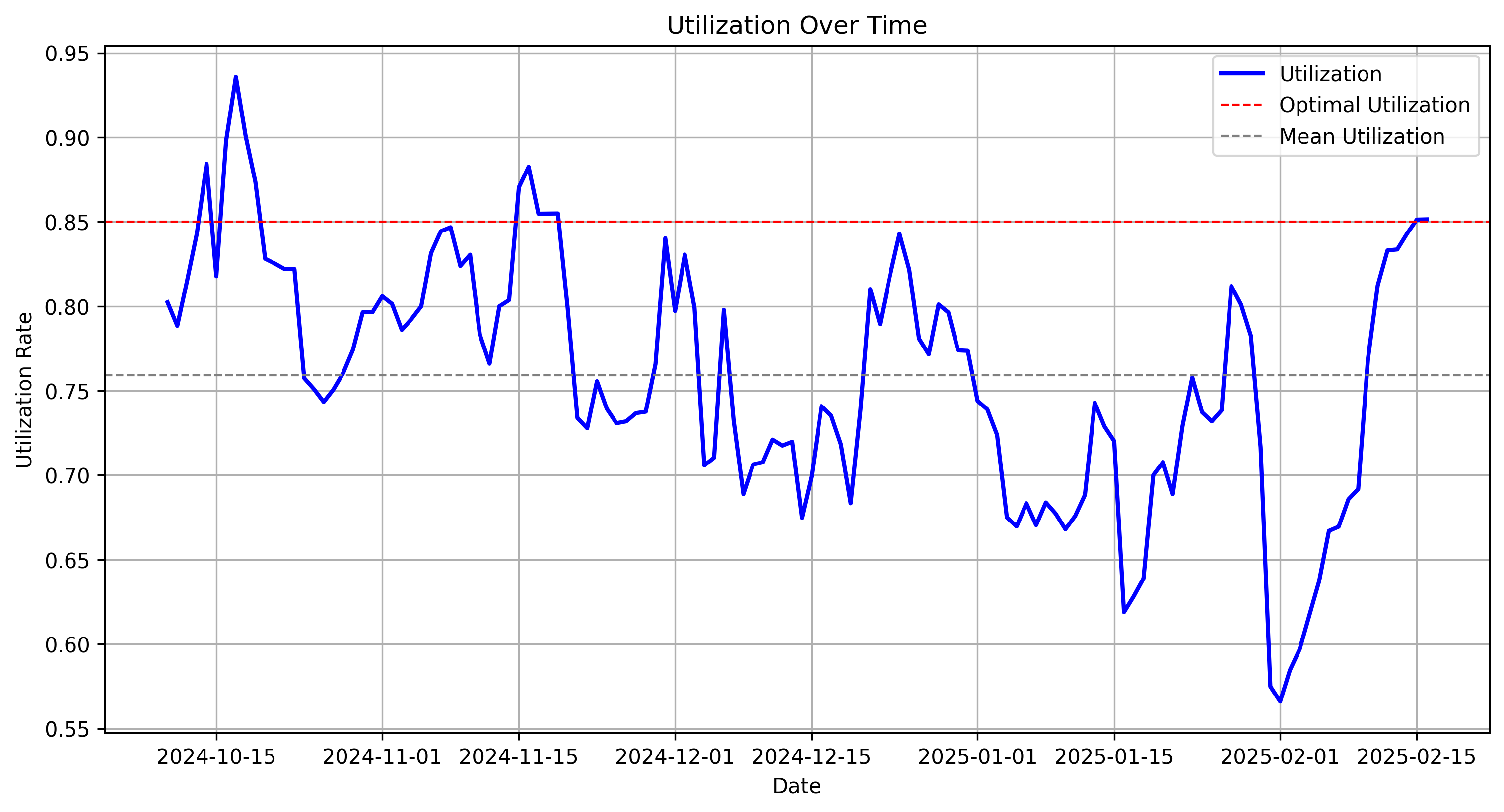
The selected regime shows, on average, a slight underutilization (76%) relative to the determined optimal level (85%).

Stochastic Parameter Estimation

We applied Ordinary Least Squares (OLS) regression to estimate parameters for our stochastic differential equation:

OLS Regression Results
==============================================================================
Dep. Variable:      delta_utilization   R-squared:                       0.065
Model:                            OLS   Adj. R-squared:                  0.057
Method:                 Least Squares   F-statistic:                     8.303
Date:                Tue, 18 Mar 2025   Prob (F-statistic):            0.00470
No. Observations:                 121   AIC:                            -527.0
Df Residuals:                     119   BIC:                            -521.5
Covariance Type:            nonrobust
==============================================================================
                 coef    std err          t      P>|t|      [0.025      0.975]
------------------------------------------------------------------------------
const          0.0197      0.007      2.703      0.008       0.005       0.034
borrow_apr_lag -0.1710      0.059     -2.881      0.005      -0.289      -0.053
==============================================================================
Omnibus:                        1.609   Durbin-Watson:                   1.818
Prob(Omnibus):                  0.447   Jarque-Bera (JB):                1.182
Skew:                           0.031   Prob(JB):                        0.554
Kurtosis:                       3.480   Cond. No.                         24.3
==============================================================================

The regression indicates a statistically significant and robust relationship. Assuming we are able to capture the response in utilization by rate for the market, currently referencing an external market through the SecondaryMP, estimates should produce a reasonable evolution of utilization paths.

Optimal Parameter Identification

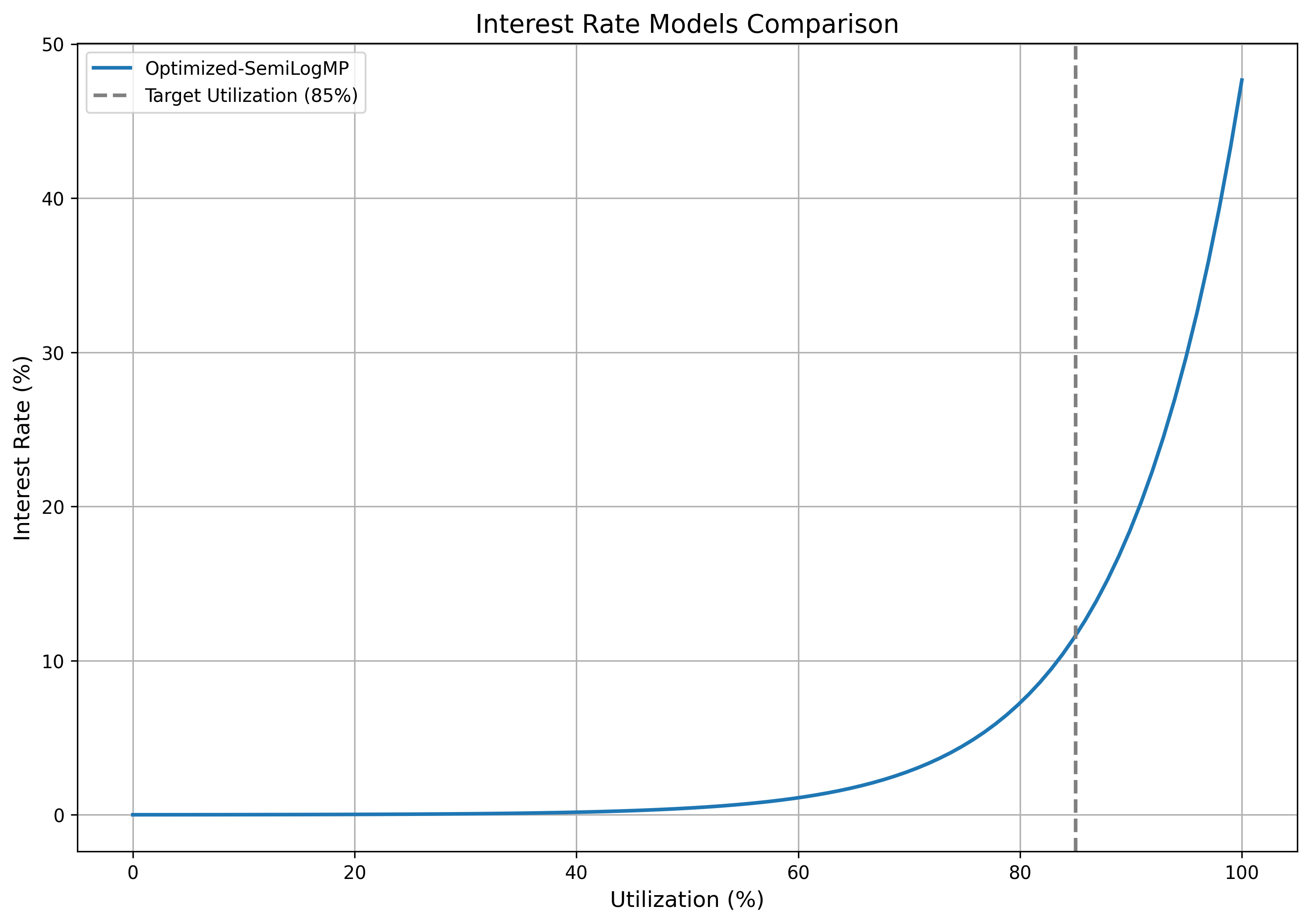
Using a composite loss function optimized over multiple stochastic simulations, we identified the following optimal parameters for the Semilog IRM:

IRM Label rate_min rate_max
Optimized-SemiLogMP 0.00004 0.47658

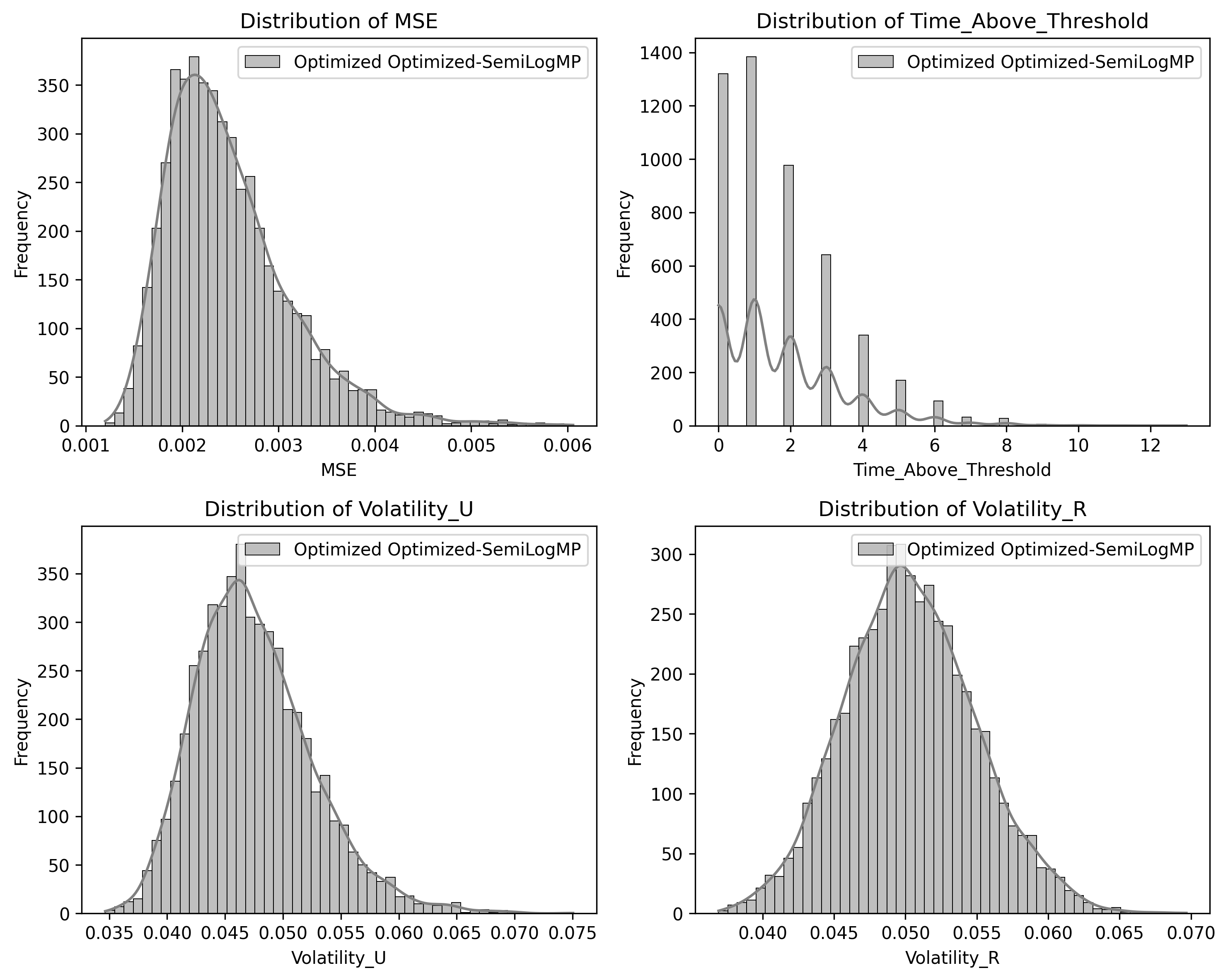
Parameter Performance Evaluation

The optimized parameters demonstrate the following performance across key metrics:

Resulting optimized interest rate curve and target utilization:

Conclusion

Switching from SecondaryMP to a semilog IRM for sUSDe offers several clear advantages:

  • Eliminates Arbitrary Rate Caps: Ensures borrowing costs can reflect actual market risk.
  • Strengthens Market Health: Encourages quicker repayment when conditions worsen, reducing the risk of illiquidity.
  • Prioritizes Lender Protection: Reduces opportunities for bad actors to exploit artificially low APRs in times of stress.

By allowing the market to determine interest rates more naturally, LlamaLend can mitigate risk effectively, preserve liquidity, and maintaining a stable lending environment—even under volatile conditions.

Specification

SUSDE_CONT = '0xB536FEa3a01c95Dd09932440eC802A75410139D6'
MONPOL = '0xb8CeDa456f8191d8D0d5b196C7BAab87A309ea50'

ACTIONS = [
    # sUSDe Sec MonPol to Semilog
    (SUSDE_CONT, "set_monetary_policy", MONPOL),
]

This vote has been started here:

At present, the market’s borrow rate is 3.53% at 76% utilization. At current utilization, the executed vote will increase the borrow rate to 5.04%. This estimate may not reflect market conditions upon vote execution next week, which may deviate due to internal market dynamics or sUSDe APR changes.

Comparing Market Performance of sUSDe: Semilog MP vs. Secondary MP

The following is a retrospective analysis on the sUSDe market following the change from Secondary to Semilog monetary policy

1. Objective

The goal of this analysis is to evaluate and compare market performance of the sUSDe Market (controller address 0xB536FEa3a01c95Dd09932440eC802A75410139D6) under two distinct Interest Rate Models (IRMs): the original Secondary Monetary Policy (Secondary MP) and the recently implemented Semilog Monetary Policy (Semilog MP). The key question addressed is whether the introduction of the Semilog MP has resulted in statistically significant changes to market stability, liquidity, and borrower behaviour.

2. Performance Metrics

We measure performance using the following metrics:

Utilization Metrics

Borrow-Rate Metrics

Liquidity and Loan Structure Metrics

3. Methodology

We employed a block bootstrap method to achieve robust, statistically valid comparisons between the two IRMs. The bootstrap approach involves repeatedly drawing random subsamples (blocks) of data from the Secondary MP period, computing performance metrics for each subsample, and then comparing these to metrics observed during the Semilog MP period. This method provides empirical distributions for each metric, allowing us to determine statistical significance without relying on parametric assumptions.

The use of block bootstrapping has several advantages:

  • It makes minimal assumptions about the underlying data distributions, which is essential given potential non-normality and autocorrelation in financial data.
  • It accounts explicitly for the temporal structure in the data by sampling contiguous blocks of days rather than independent daily observations, preserving dependencies inherent in market data.
  • It allows estimation of confidence intervals, enabling robust significance testing.

Achieving significance:

Statistical significance is established by comparing observed Semilog MP metrics to the empirical distribution derived from bootstrap samples of Secondary MP. Metrics are considered statistically significant if the Semilog MP value falls outside the 95% confidence interval (2.5% – 97.5%) of the Secondary MP bootstrap distribution.

Key assumptions and potential limitations:

  • The primary assumption underlying bootstrap comparability is that the Secondary MP historical environment accurately represents potential market conditions under Semilog MP.
  • By matching yield environments explicitly in the second analysis, we attempt to control for macroeconomic influences that could confound IRM effects. However, exact comparability can still be affected by other unaccounted-for market factors such as liquidity shocks, external market volatility, or changes in borrower behavior unrelated to IRM structures.
  • Any systematic differences in these uncontrolled factors could partially violate direct comparability, making interpretation reliant on careful contextual judgment.

Block Samples
Below we display which segement qualify as sampling regions based on comparable yield regime for the regime specific bootstrap sampling:

4. Results

This section presents a comparative evaluation of the proposed Secondary Monetary Policy (MP) against the baseline Semilog MP across two simulation environments: a broad, unconditional environment and a yield-matched, conditional environment. Metrics are reported with 95% confidence intervals derived from bootstrapped simulations of the Secondary MP, while Semilog MP values are point estimates from a fixed policy.


Utilization

Table I: Utilization Metrics - Broad Environment Results (unconditional):

Metric Secondary MP (95 % CI) Semilog MP Significant?
Utilisation volatility 0.029 – 0.138 0.027 Yes
Utilisation CV 0.030 – 0.212 0.0396 No
Utilisation IQR 0.033 – 0.175 0.0371 No
Utilisation MAC 0.0070 – 0.0578 0.0193 No

Table II: Utilization Metrics - Yield‑Matched Environment Results (conditional)

Metric Secondary MP (95 % CI) Semilog MP Significant?
Utilisation volatility 0.0229 – 0.0753 0.0270 No
Utilisation CV 0.0254 – 0.0922 0.0396 No
Utilisation IQR 0.0138 – 0.124 0.0371 No
Utilisation MAC 0.0054 – 0.0189 0.0193 Yes

In the broad environment, Table I, the Secondary MP leads to significantly higher utilization volatility (0.029–0.138) compared to Semilog MP (0.027), suggesting that it introduces more unpredictable engagement from suppliers and borrowers. However, the Coefficient of Variation (CV) and Interquartile Range (IQR)—which reflect normalized and robust dispersion—show no significant difference, indicating that relative and typical utilization patterns remain stable. The Mean Absolute Change (MAC), a proxy for daily jitter, is also statistically similar, implying that short-term reactivity under both policies is comparable.

In the yield-matched environment, Table II, volatility differences shrink and become statistically insignificant, suggesting that the Secondary MP can stabilize utilization when rate incentives are controlled. The utilization MAC is (significantly) lower, indicating smoother, less reactive market dynamics—a desirable outcome for predictable system behaviour.


Borrow Rate

Table III: Borrow Rate Metrics - Broad Environment Results (unconditional):

Metric Secondary MP (95 % CI) Semilog MP Significant?
Borrow‑rate volatility 0.0067 – 0.0392 0.0059 Yes
Borrow‑rate CV 0.100 – 0.427 0.225 No
Borrow‑rate IQR 0.0046 – 0.0686 0.0071 No
Borrow‑rate MAC 0.0016 – 0.0147 0.0042 No

Table VI: Borrow Rate Metrics - Yield‑Matched Environment Results (conditional)

Metric Secondary MP (95 % CI) Semilog MP Significant?
Borrow‑rate volatility 0.0050 – 0.0150 0.0059 No
Borrow‑rate CV 0.077 – 0.264 0.225 No
Borrow‑rate IQR 0.0015 – 0.0262 0.0071 No
Borrow‑rate MAC 0.0011 – 0.0058 0.0042 No

In the broad environment, Table III, the Secondary MP results in significantly higher borrow-rate volatility (0.0067–0.0392) relative to the Semilog MP (0.0059), suggesting less predictable borrowing costs under the adaptive policy. However, no significant differences are observed in the Coefficient of Variation (CV), Interquartile Range (IQR), or Mean Absolute Change (MAC). This implies that while rates may fluctuate more overall, their relative variability, central spread, and day-to-day changes remain within acceptable bounds, preserving general borrowing conditions.

In the yield-matched environment, Table VI, none of the borrow-rate metrics differ significantly. Volatility, CV, IQR, and MAC all fall within overlapping confidence intervals. This indicates that when the reference yield is held constant, the Secondary MP delivers comparable rate stability to the Semilog MP — given both have similar shapes this may explain this phenomena.


Lending Market
Table V: Lending Market Metrics - Broad Environment Results (unconditional):

Metric Secondary MP (95 % CI) Semilog MP Significant?
Liquidity buffer (USD) 0.21 M – 1.92 M 4.05 M Yes
Loan‑count volatility 0.00 – 3.40 6.15 Yes
Average loan size (USD) 0.279 M – 0.523 M 0.241 M Yes
CV loan size 0.0010 – 0.273 0.153 No

Table IV: Lending Market Metrics - Yield‑Matched Environment Results (conditional):

Metric Secondary MP (95 % CI) Semilog MP Significant?
Liquidity buffer (USD) 0.21 M – 0.401 M 4.05 M Yes
Loan‑count volatility 0.00 – 0.509 6.15 Yes
Average loan size (USD) 0.332 M – 0.396 M 0.241 M Yes
CV loan size 0.0007 – 0.0861 0.153 Yes

In the broad environment, Table V, the Secondary MP yields a much lower liquidity buffer (0.21 M–1.92 M) compared to the Semilog MP (4.05 M). This is accompanied by a significantly lower loan-count volatility (0.00–3.40 vs. 6.15), suggesting that borrower activity is more stable under the adaptive policy. The average loan size is significantly higher under Secondary MP, which may reflect a concentration of debt among fewer borrowers, though the coefficient of variation (CV) for loan sizes is not significantly different—implying that loan size dispersion is preserved overall. In the yield-matched environment, Table VI the same patterns hold but are more pronounced, except the CV is significantly higher. Overall, we need to be critical of these results as the introduction of Resupply to the market led to a rapid increase in in total asset supplied and borrowed.


5. Conclusion

The analysis demonstrates:

  • Utilization & Rate Stability: Improvements in volatility metrics observed under Semilog MP in the broad environment were largely due to different yield conditions. After yield matching, these benefits disappear, suggesting yield, rather than the IRM itself, influenced stability. This makes sense as both curves in a static environment have a similar shape.
  • Short‑term utilisation jitter increases under Semilog. Mean‑absolute‑change (MAC) in utilisation is significantly higher only in the yield‑matched comparison, implying that once we hold the yield backdrop constant, Semilog MP induces more day‑to‑day adjustment noise.

    Note: This threshold just about satisfies the significance level.

  • Liquidity Management: Semilog MP consistently provided a significantly larger liquidity buffer, independent of yield environment. Yet, given this occured during a period where Resupply launched, liquidity buffer cannot be attributed to the policy itself.
  • Borrower Dynamics: Under Semilog MP, loan-count volatility and loan-growth rates significantly increased, indicating higher borrower activity and churn. Additionally, loans became smaller and more unevenly sized, dispersing risk across more borrowers but creating greater variability. Again, this likely results from the introduction of Resupply rather than the switch in policy itself.

In conclusion, Semilog MP does not improve fundamental market stability when controlling for yield environment. These results yielded from this study were unable to highlight clear benefits of the SemiLog MP over the Secondary MP in the studied aspects. We recommend to re-do the analysis at a later point in time, when more data is available for sUSDe under a Semilog policy.

As an additional resource following the enactment of this Monetary Policy change, we present some data about the respective markets’ behavior, highlighting the date when the policy change was enacted

The on-chain vote that was initiated on 3/19 to the Curve DAO sought to adjust the monetary policy for the sUSDe-long-v2 Llamalend market from Secondary Policy to Semilog with min/max rate 0.004%/47.658%. In the resulting graphs, the first dotted red line is when the proposal was introduced and the second line being when the monetary policy was enacted.

image
image
image
image