Summary
Change min/max borrow rate parameters on the sDOLA LlamaLend Monetary Policy from 0.5%/15% to 0.1%/25%.
Motivation
The sDOLA-long market was deployed on ethereum with the controller address:
0xCf3DF6C1B4A6b38496661B31170de9508b867C8E.The current Interest Rate Model (IRM) is SemiLogIRM, with the following parameters:
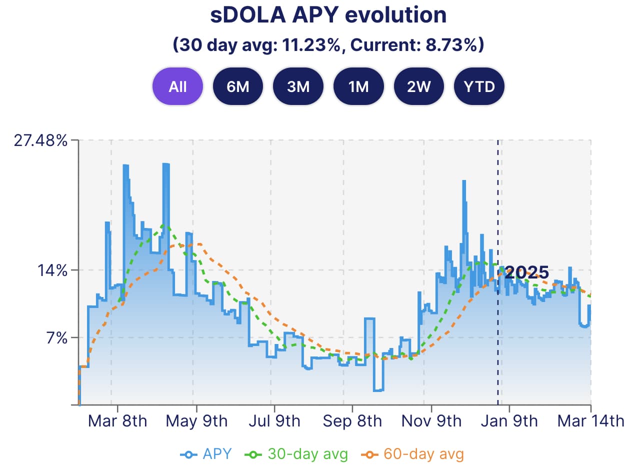
min_rate= 0.005max_rate= 0.15The min/max parameters in the LlamaLend Semilog Monetary Policy set the bounds charged to borrowers depending on the utilization of the market. In stablecoin lending markets such as sDOLA, borrowers seek to leverage exposure to the sDOLA yield, and therefore borrow demand should be sensitive to changes in the sDOLA yield. In cases where yield persistently exceeds 15%, the market may be at risk of illiquidity. The evolution of sDOLA APY demonstrates that there is a reasonable possibility of yields that exceed the LlamaLend market’s bounds.
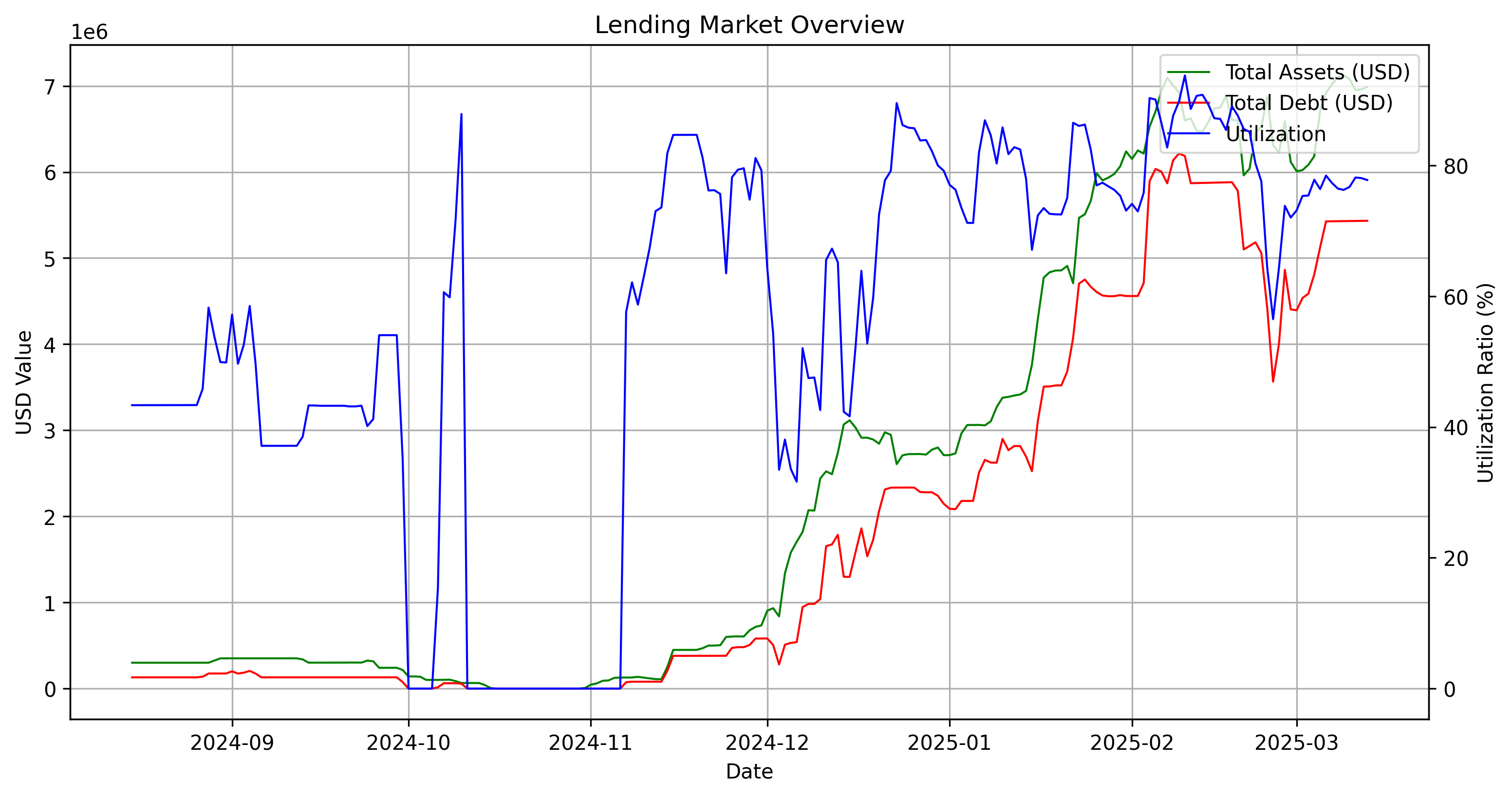
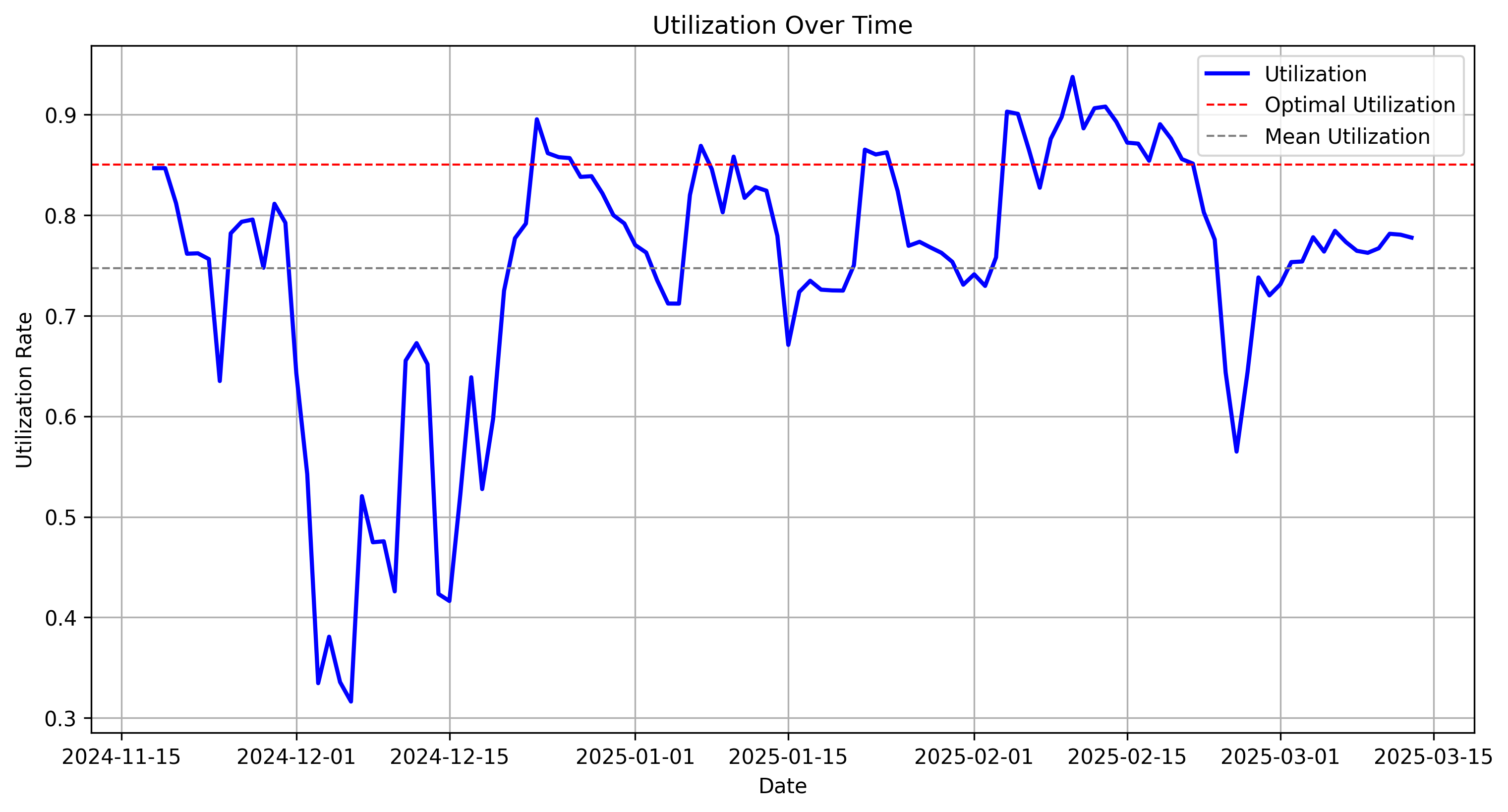
This plot below compares total assets and total debt over time while overlaying utilization on a secondary axis.
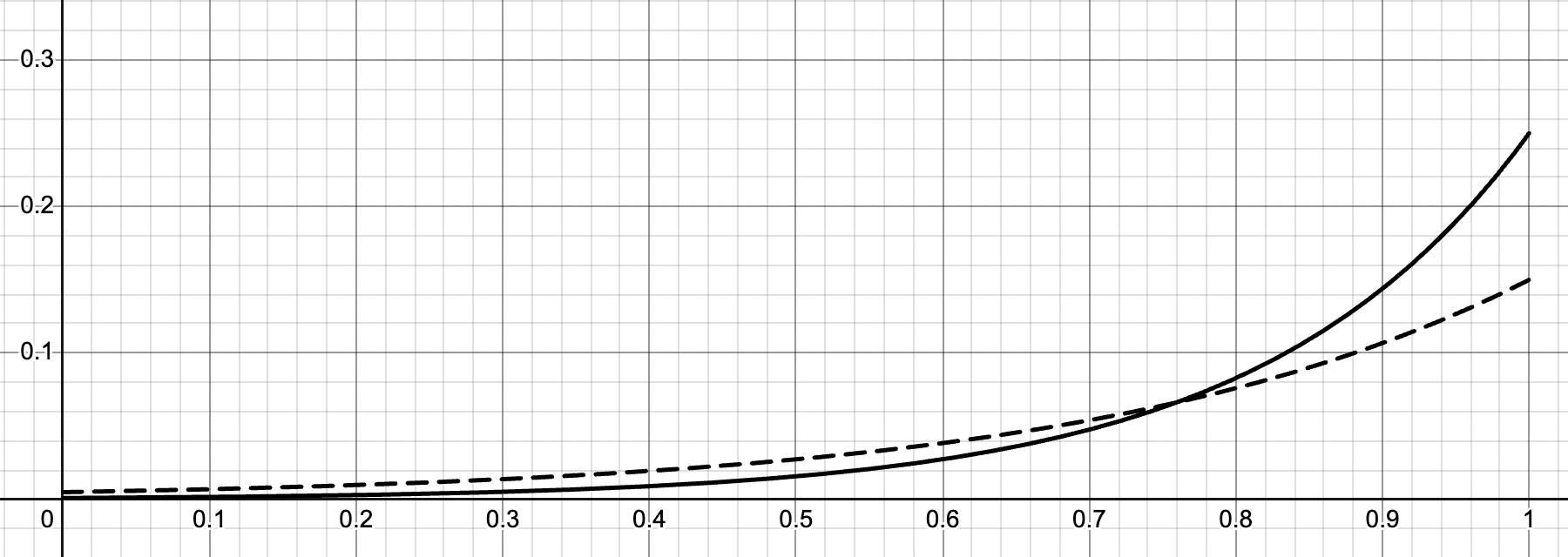
Our goal with this proposal is to adjust the rate parameters such that there is additional buffer on the max rate to avoid periods of illiquidity, while minimizing impact to the market’s rates and avoiding excessive rate volatility. See below the current IRM curve (dashed line) and the proposed IRM curve (solid line), plotting market utilization on the x axis and borrow rate on the y axis.
Given below, for academic interest, is an optimization analysis we have done for sDOLA. It’s produces a recommendation with a wider spread, so we rather prefer a more gradual adjustment. This analysis offers insight into our priorities and process when determining optimal parameters and suggests our target for future adjustments to the sDOLA market.
sDOLA-long Analysis
Optimal Utilization Analysis
We identify volatile periods based on the price oracle feed and then analyze the withdrawal quantile of total assets during these periods.
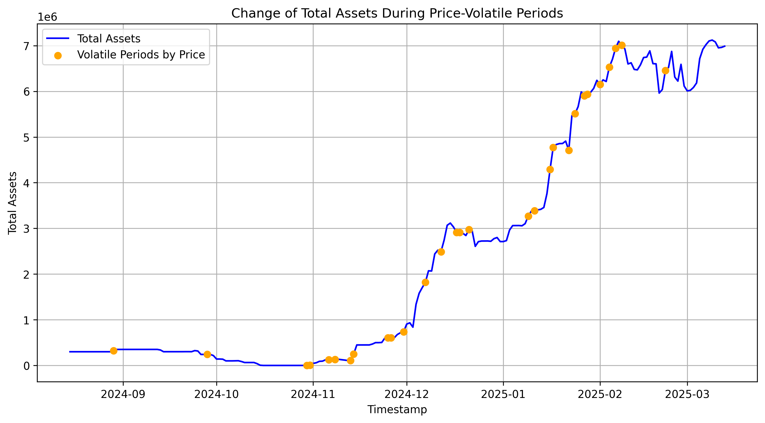
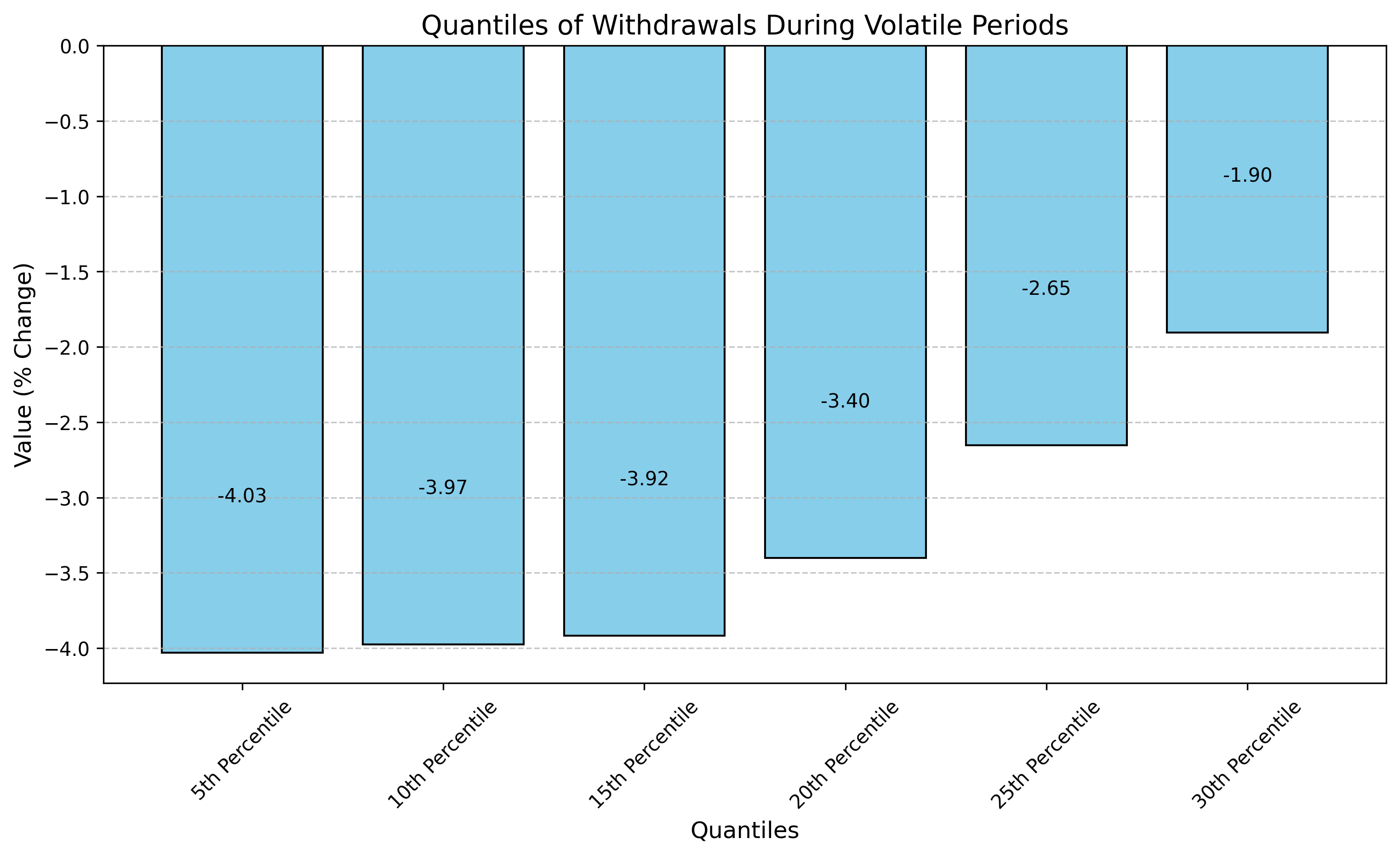
The 10th percentile of negative withdrawals of supplied crvUSD during volatile periods was 3.99% of the total supply.This means that 90% of all observed withdrawals during volatile periods were less than or equal to this value. Given that optimal utilization is defined as min(1- withdrawal_quantile, 0.85), optimial utilization is 85%.
Regime Shift Analysis
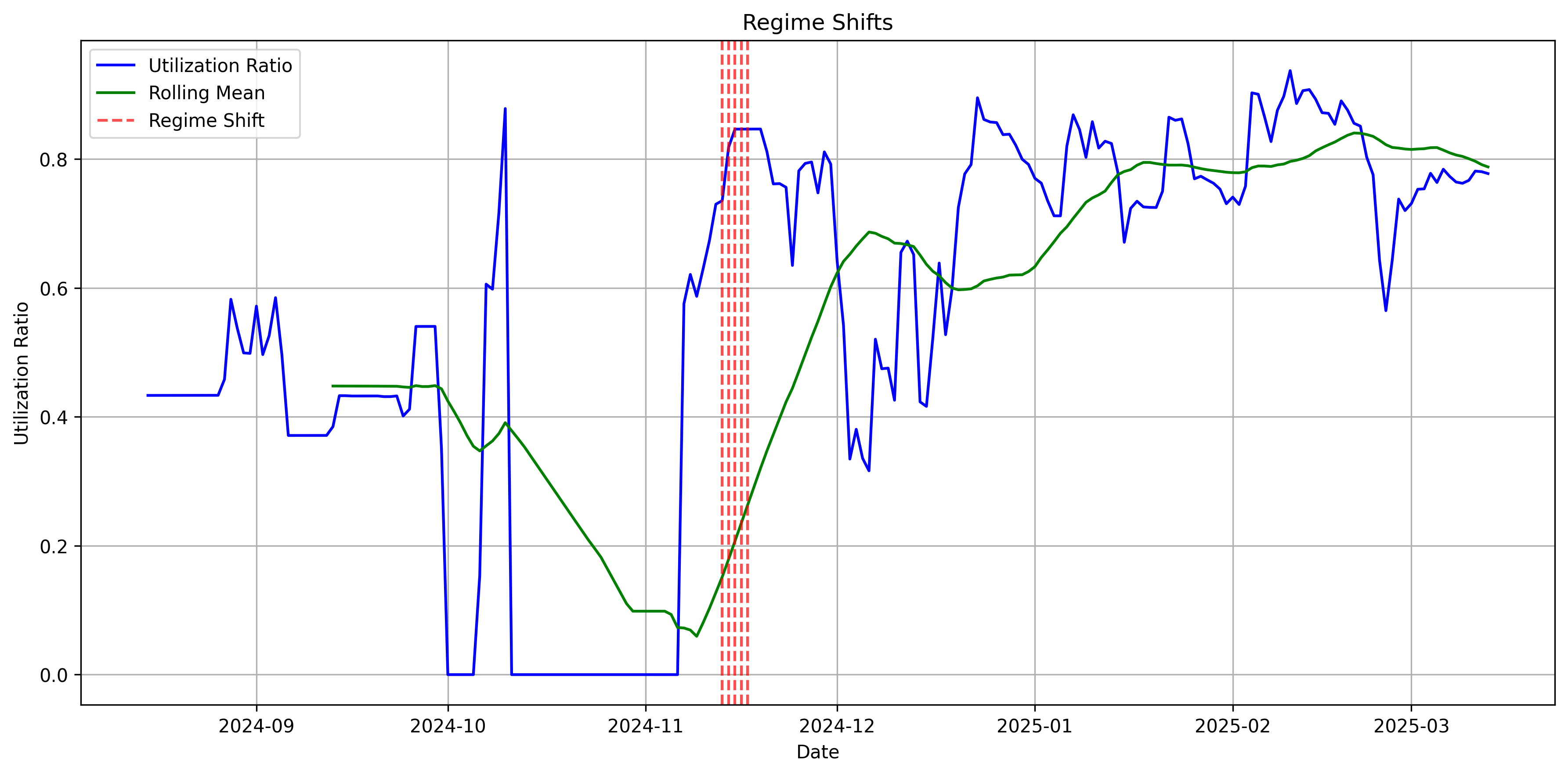
This plot shows detected regime shifts in utilization. Red vertical lines indicate significant shifts, which represents changes in stability in utilization in this given market.
The latest stable regime shift was detected on 2024-11-17.We ended observation on 2025-03-13, covering a period of 116 days.
The regime can be categorized as being underutilized- an average 75% utilization observed is below our target of 85%.
Parameterizing of the underlying Model
We estimate underlying model parameters for the Stochastic differential equation using a simple OLS model.
OLS Regression Results
==============================================================================
Dep. Variable:      delta_utilization   R-squared:                       0.050
Model:                            OLS   Adj. R-squared:                  0.041
Method:                 Least Squares   F-statistic:                     5.566
Date:                Thu, 13 Mar 2025   Prob (F-statistic):             0.0202
Time:                        14:33:39   Log-Likelihood:                 182.09
No. Observations:                 107   AIC:                            -360.2
Df Residuals:                     105   BIC:                            -354.8
Df Model:                           1
Covariance Type:            nonrobust
==================================================================================
                     coef    std err          t      P>|t|      [0.025      0.975]
----------------------------------------------------------------------------------
const              0.0305      0.014      2.192      0.031       0.003       0.058
borrow_apr_lag    -0.4386      0.186     -2.359      0.020      -0.807      -0.070
==============================================================================
Omnibus:                        5.315   Durbin-Watson:                   1.927
Prob(Omnibus):                  0.070   Jarque-Bera (JB):                7.782
Skew:                           0.055   Prob(JB):                       0.0204
Kurtosis:                       4.317   Cond. No.                         43.4
==============================================================================

Notes:
[1] Standard Errors assume that the covariance matrix of the errors is correctly specified.
Validating the Underlying Model
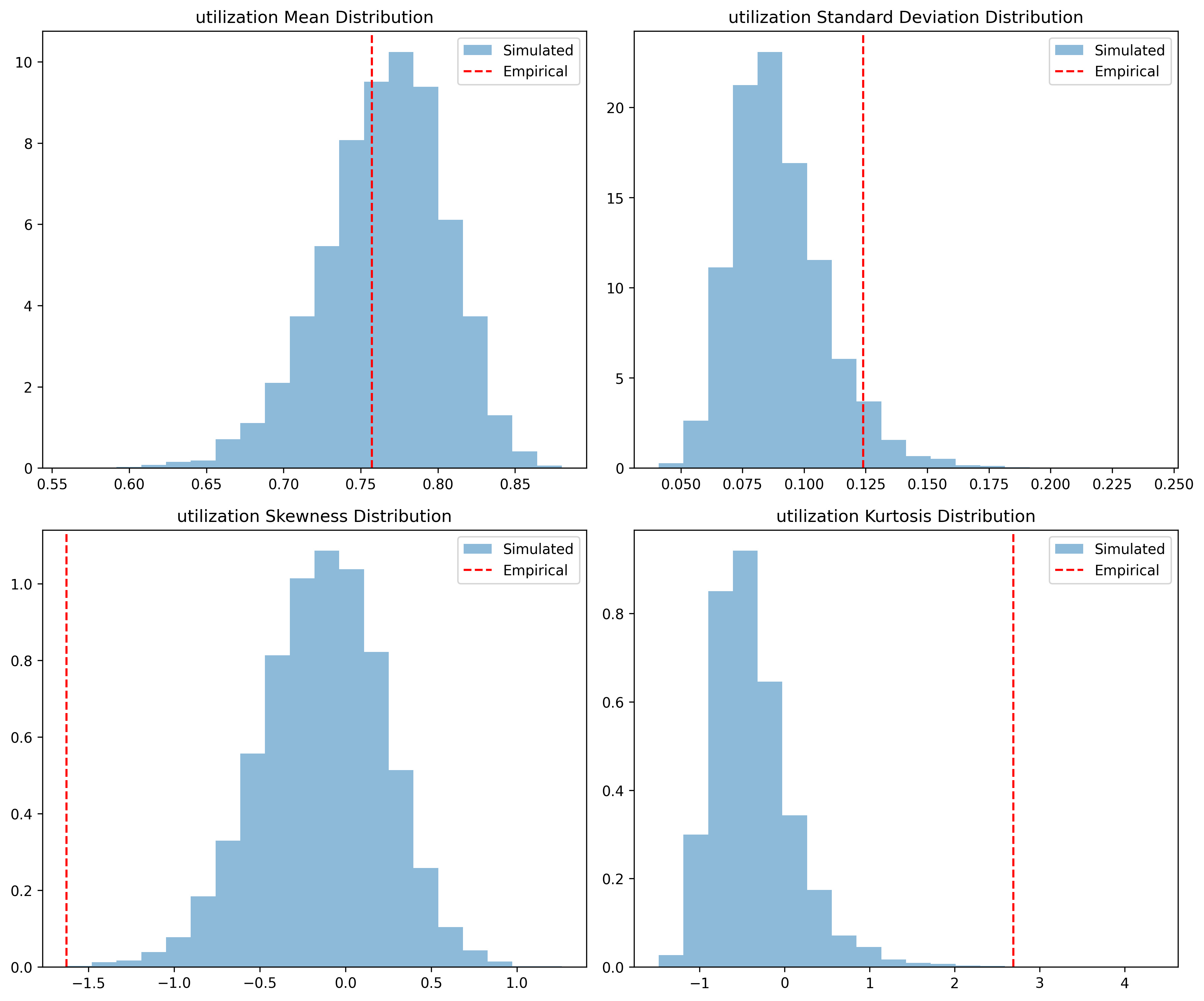
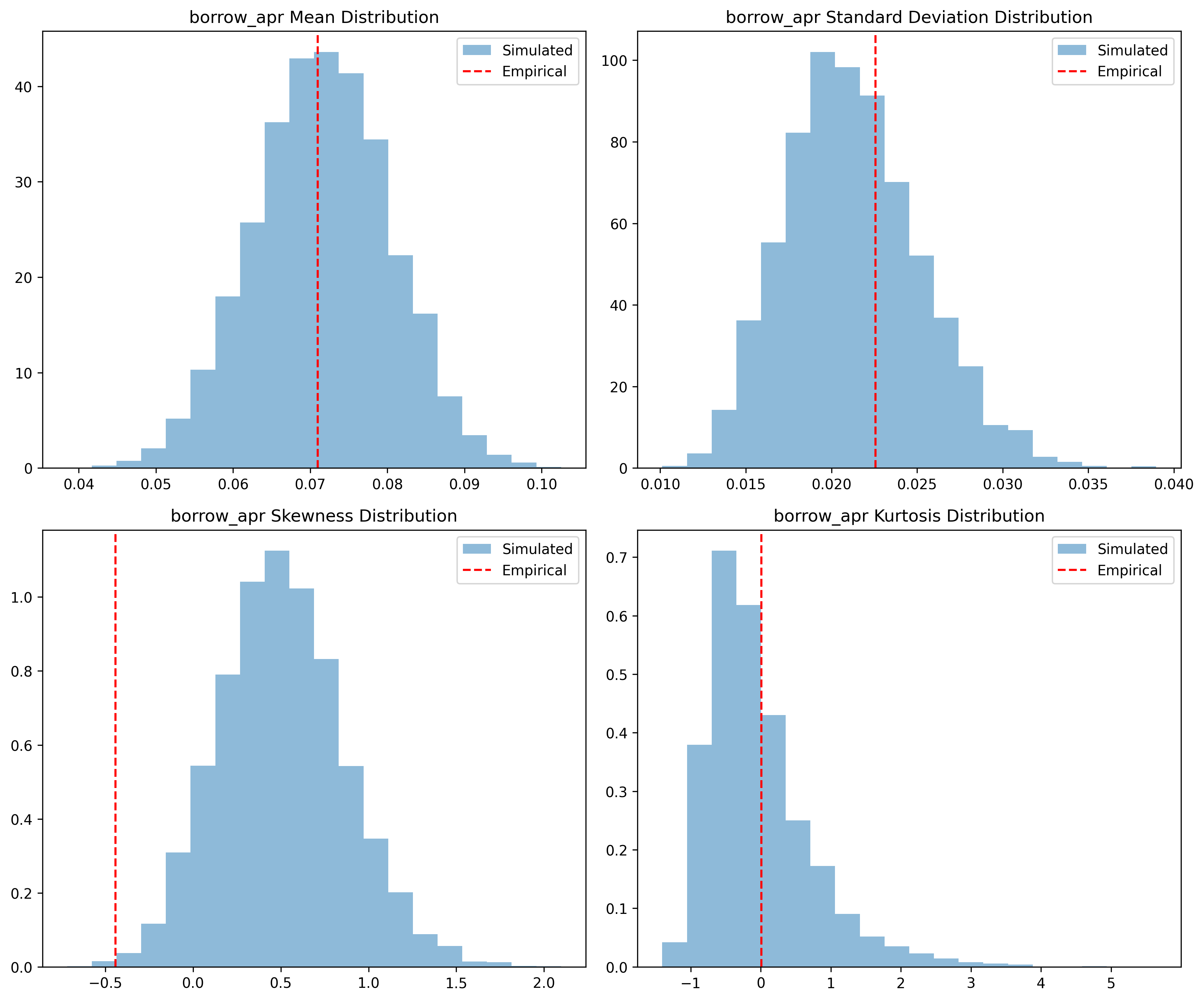
The plot above visualizes the distribution of key statistical metrics for empirical vs. simulated utilization. Red lines mark empirical values, allowing direct comparison with simulated distributions.
Rate Table
| Metric | Empirical Value | Simulated Value |
|---|---|---|
| Mean | 0.0710 | 0.0715 |
| Std Dev | 0.0226 | 0.0213 |
| Skewness | -0.4427 | 0.5079 |
| Kurtosis | 0.0081 | -0.0273 |
Utilization Table
| Metric | Empirical Value | Simulated Value |
|---|---|---|
| Mean | 0.7571 | 0.7651 |
| Std Dev | 0.1239 | 0.0902 |
| Skewness | -1.6288 | -0.1394 |
| Kurtosis | 2.6912 | -0.3694 |
These tables compare empirical and simulated values for utilization and rates. A large difference in mean utilization or rate indicates a potential issue with the simulation. We can see that in particular the utilization standard deviation is slighlty underestimated in our model.
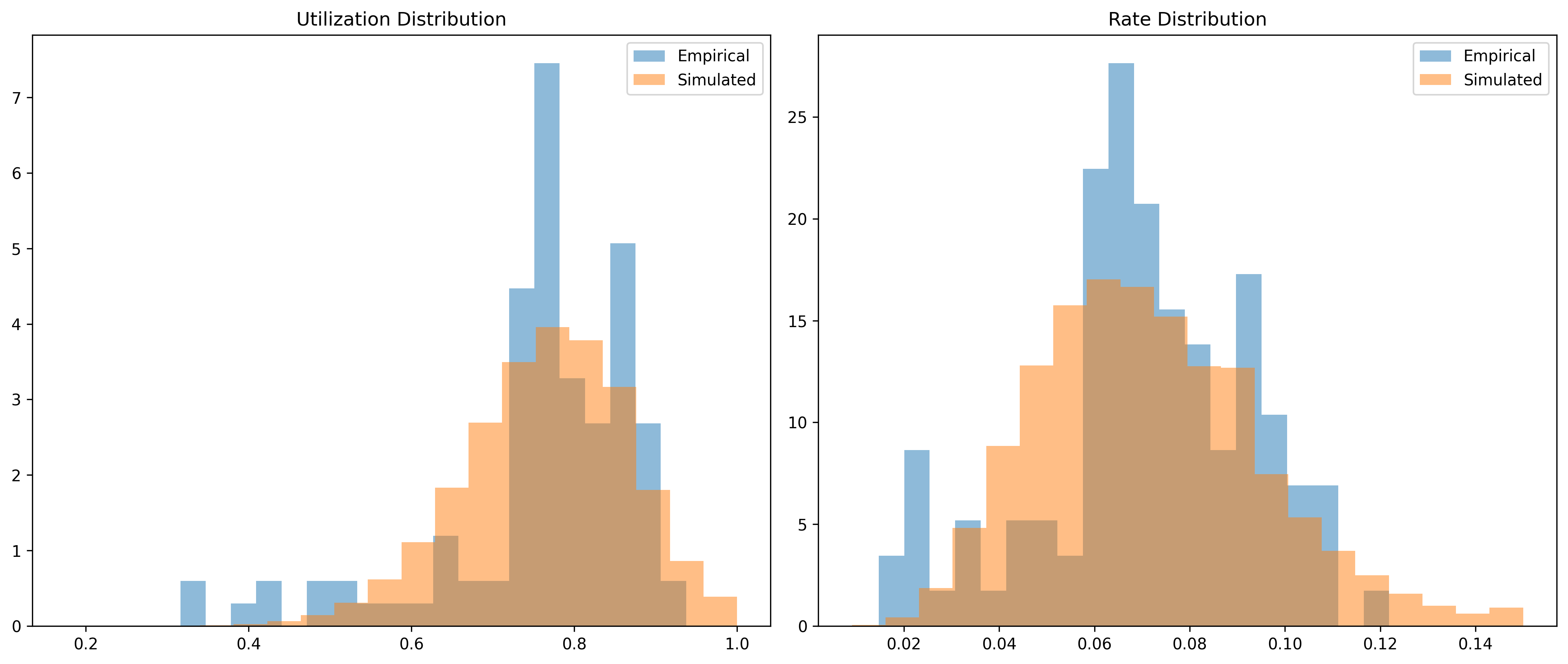
This plot compares the empirical and simulated distributions of utilization and rates. A close match indicates realistic simulation dynamics.
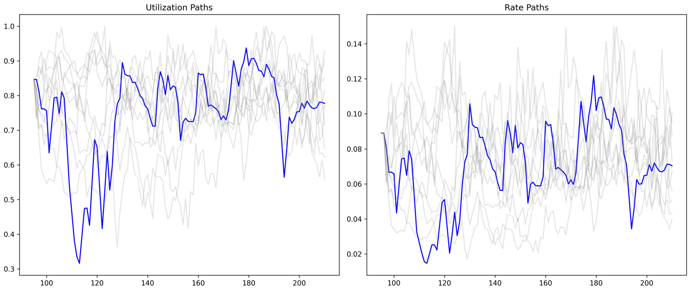
This plot compares real utilization and rate paths with simulated ones. Gray lines represent simulated paths, while blue lines show empirical values.
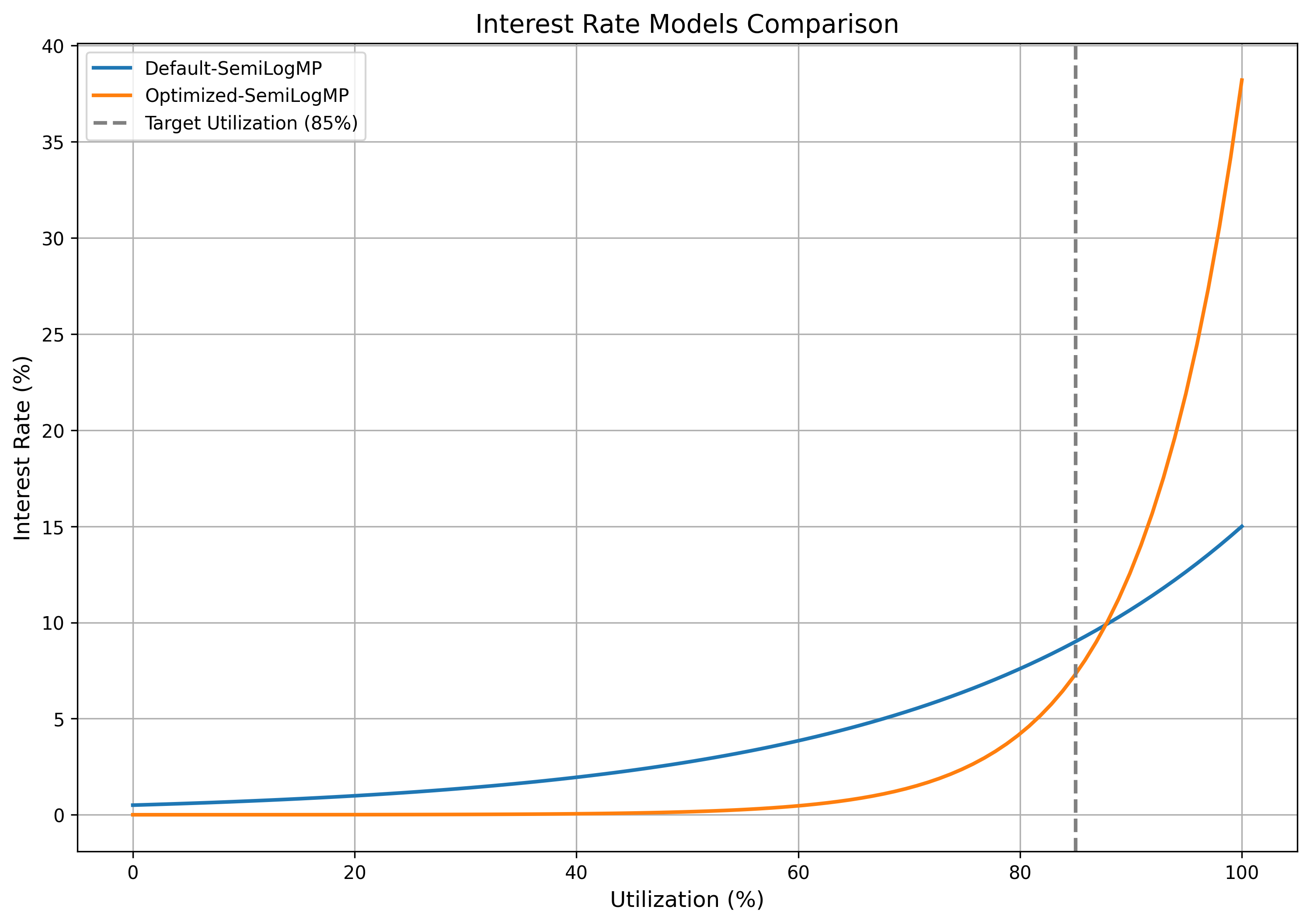
Optimal Parameters
After optimizing with the composite loss function (as specified in the methodology) across multiple simulated SDE paths, we identified the optimal parameters as:
| IRM Label | rate_min | rate_max |
|---|---|---|
Optimized-SemiLogMP |
0.00001 |
0.38211 |
Evaluating Parameter Performance
In this section, we compare the default configuration of parameters with the optimized parameters across key performance metrics.
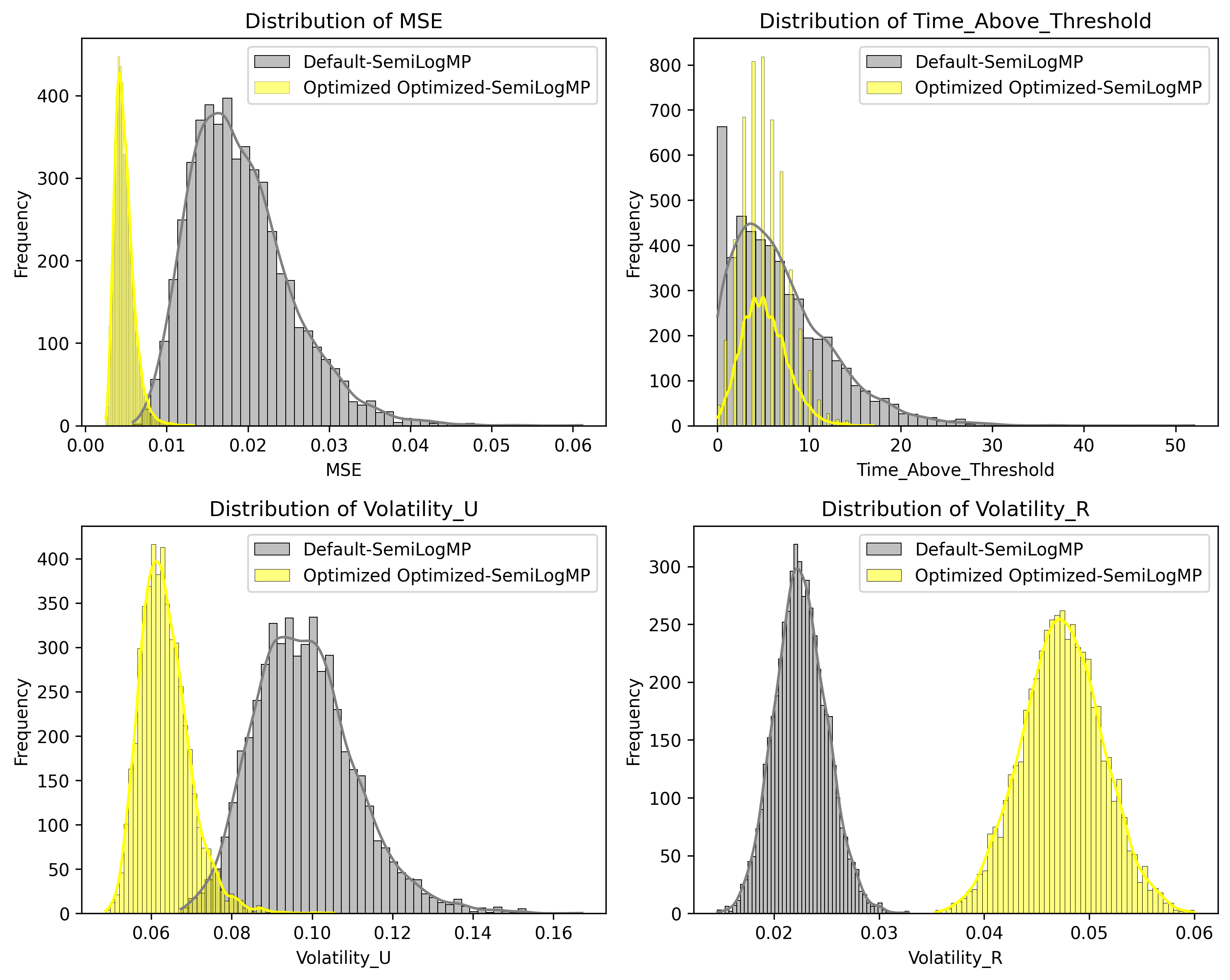
The chart suggests that:
- Mean Squared Error (MSE) is lower for the Optimized Model, hence it trades closer to the optimal utilization level defined.
- Time Above Threshold is lower for the optimized model.
- The Volatility of the Utilization is lower on the Optimized model suggesting stability in utilization level
- The Volatility of the Rate is higher which as uncovered before mark the fundamental trade-off to manage rates effectively.
Conclusion
The Optimized Model consistently outperforms the default configuration, balancing trade-offs between rate volatility and MSE.
Specification
Call the sDOLA LlamaLend Monetary Policy contract.
ACTIONS = [
    # sDOLA min/max rate 0.1%/25%
    ("0x0b10DD6Be465bC21E057FAf8b05B61dE8DB070F0", "set_rates", 31709791, 7927447995),
]
For:
Adjusted parameters provide stronger assurances to lenders that the IRM can preserve market liquidity in periods of high borrow demand
Against:
Increased min/max spread increases the rate sensitivity of the IRM curve.