Executive Summary
This analysis provides parameter recommendations for the new stLINK/LINK StableSwap-NG Curve pool, examining both current market conditions and projected scenarios with enabled withdrawals. Stake.link plans to implement stLINK withdrawal functionality within 1-2 weeks. The multisig to roll out native withdrawals is live now, so Stake.link expect that native withdrawals will be live by the time pool liquidity is migrated. This will fundamentally change the asset’s peg behavior by introducing a direct arbitrage path.
We expect the introduction of withdrawals to reduce the spread between stLINK and LINK for several reasons:
- The direct redemption mechanism provides a more efficient arbitrage path for downside deviations
- Historical data shows consistent staking activity despite capacity restrictions on the staking pool, with 172k LINK staked in the last 30 days
However, this mechanism operates within certain constraints:
- The LINK staking pool has a cap that historically tends to be completely filled. While withdrawals will help reinforce the downside peg through arbitrage, upward price pressure may persist due to limited staking capacity.
- When stLINK trades at a premium, holders are incentivized to sell the premium and redeposit LINK to stLINK. However, this process is not instant due to the queuing system for new stakes. The protocol maintains a pool of LINK waiting to be staked, depositing to the staking pool whenever there is capacity (via MEV bot).
- The withdrawal system allows for a maximum 25% of the underlying LINK to be withdrawn per week. While such extreme withdrawal demand is unlikely to be realized, it does represent a limitation in the withdrawal system’s capacity to facilitate timely peg arbitrage.
Given these dynamics, our analysis emphasizes optimizing liquidity depth while acknowledging that sustained upward depegs may be more likely than downside deviations. Since the pool’s primary purpose is to provide exit liquidity for stLINK, upward depegs can be considered more tolerable as they increase the proportion of LINK available in the pool.
Our recommendations are based on simulations under both current conditions and projected (reduced spread) scenarios, accounting for these structural characteristics of the asset. We provide optimization recommendations for the liquidity concentration (Amplification coefficient), the base swap fee (Base fee), and the fee multiplier when offpeg.
| Parameter | Current Environment | After Withdrawal Implementation |
|---|---|---|
| Amplification Coefficient (A) | 200-300 | 500 |
| Base fee | 1000000 (0.01%) | 1000000 (0.01%) |
| Offpeg Fee Multiplier | 5x | 5x |
Methodology & Analysis Results
Our analysis employed simulation-based modeling to evaluate pool performance under varying market conditions. We conducted two primary simulation sets:
1. Current Market Environment Analysis
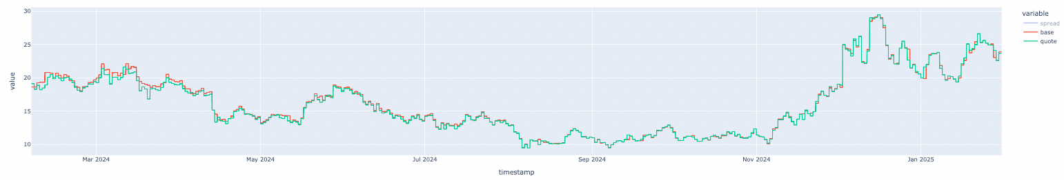
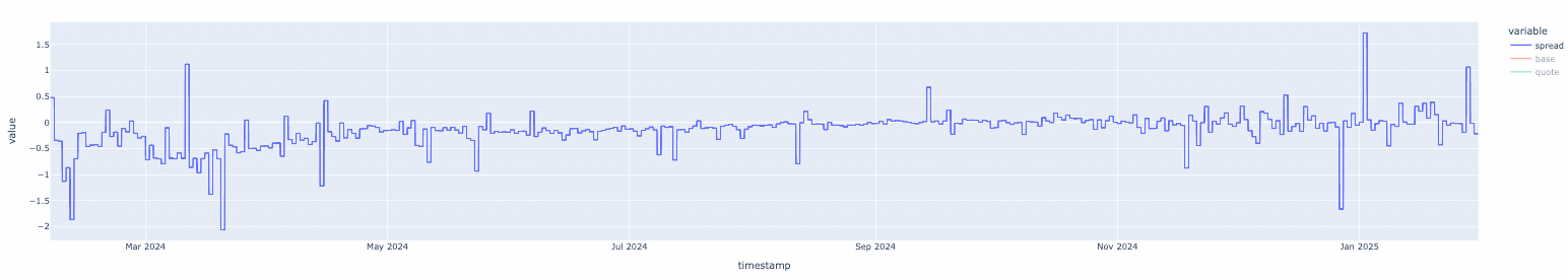
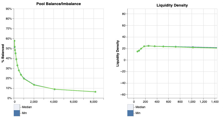
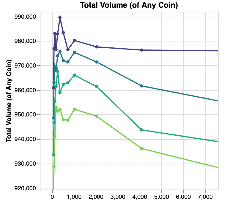
The first simulation set analyzed pool behavior under current spread conditions. In the following charts we can visualize the price and historical spread of LINK/stLINK.
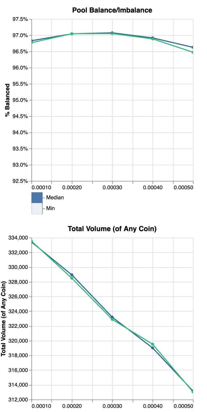
We conduct simulation runs of the the assets’ historical price path across a parameter set of various pool concentrations (amplification coefficient, or “A” parameter) and pool swap fees. By simulating arbitrage in the pool, we can observe the influence that different parameter configurations have on critical pool performance factors like pool balance, liquidity density, and arbitrage volume.
Results indicated that an amplification coefficient between 200-300 provides optimal balance between capital efficiency and stability. At this range, liquidity density is minimized and volume is maximized, indicating that this liquidity concentration ensures optimal pool performance. Higher values would increase slippage during larger trades and potentially destabilize the pool during high volatility periods.
x-axis: A
Note: Each curve in the charts above is associated with the following fee value:

The decrease in volume with excessive A values can be attributed to two main factors. First, when A becomes very high, the curve becomes so flat that arbitrage profits become minimal, reducing incentives for arbitrageurs to trade. Second, excessive A values result in over-concentration of liquidity around the current price point, making the pool less efficient for trades when prices move significantly from equilibrium. This inefficient liquidity may ultimately result in lower overall volume.
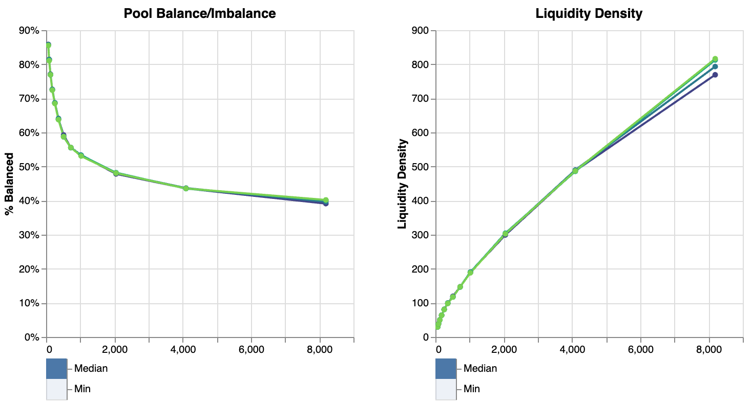
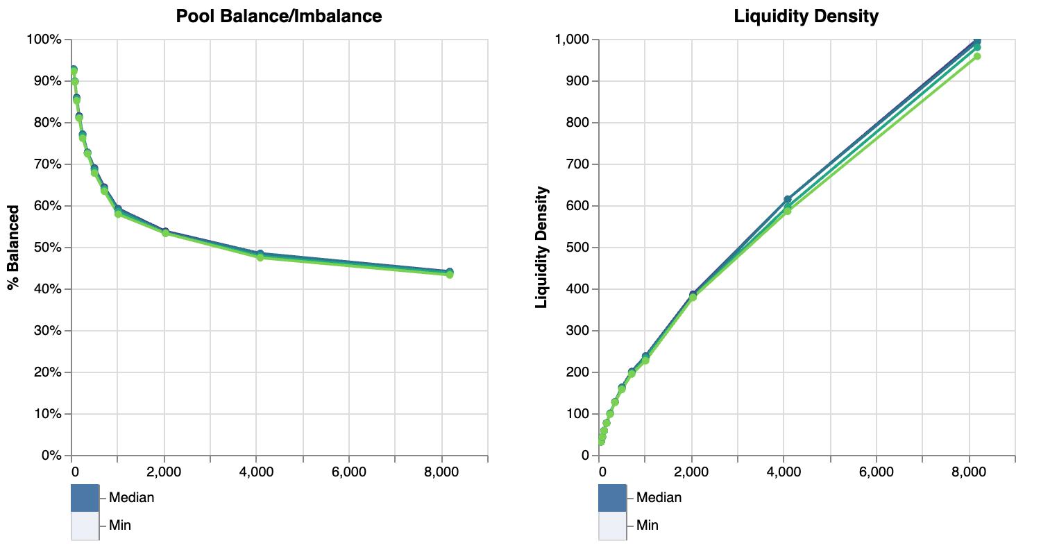
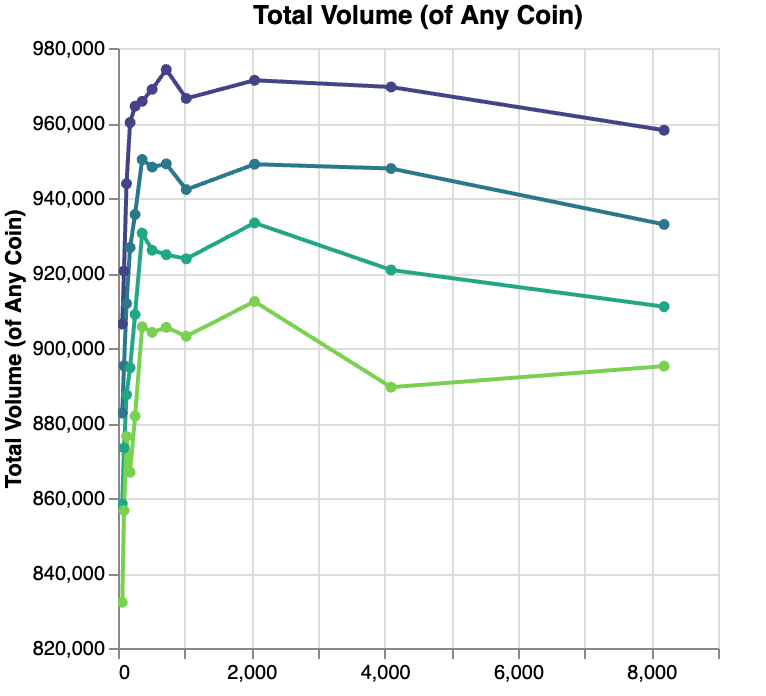
2. Reduced Spread Scenario Analysis:
The second simulation set examined pool behavior with an assumed 50% reduction in spread, anticipating the implementation of withdrawals. Under these conditions, the pool demonstrated capacity for higher capital efficiency.
The simulations showed that amplification coefficients between 800-1000 become potentially viable, significantly improving liquidity density without compromising stability. Arbitrage volume is maximized and minimum liquidity depth is minimized in the range from 400-800. Given that the actual peg behavior of stLINK after enabling withdrawals cannot be fully assessed, a reasonable A value should prefer the slightly more conservative stance. A=500 should offer good operational performance at pool deployment, and further refinement to the liquidity concentration can be done after the pool has time to mature.

Note: Each curve in the charts above is associated with the following fee value:
Fee Structure Analysis
Our simulations indicated that reducing the base fee to 1000000 (0.01%) would optimize pool volumes.
The offpeg_fee_multiplier determines how much the fee increases when assets within the AMM depeg. Our recommendation is to set this value at 5x, which provides additional compensation to liquidity providers during off-peg scenarios. The multiplier can partially offset the reduced pool returns from the lower base fee. This assures competitive trading conditions during normal operations without forfeiting potential fee revenue in volatile market scenarios.
x-axis: fee